Table of contents
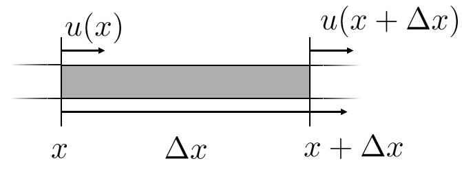
If we take a look at a so called infinitesimal element of size Δ x \Delta x Δ x x x x u ( x ) u\left(x\right) u ( x ) x + Δ x x+\Delta x x + Δ x u ( x + Δ x ) u\left(x+\Delta x\right) u ( x + Δ x )
ε : = e l o n g a t i o n o r i g i n a l l e n g t h = u ( x + Δ x ) − u ( x ) Δ x → d u d x \varepsilon :=\dfrac{\mathrm{elongation} }{\mathrm{original} \mathrm{length} }=\dfrac{u\left(x+\Delta x\right)-u\left(x\right)}{\Delta x}\to \dfrac{d u}{d x} ε := original length elongation = Δ x u ( x + Δ x ) − u ( x ) → d x d u In 1D the relation between the strain and stress is done using the linear elasticity modulus (tensile modulus or Young's modulus) E E E
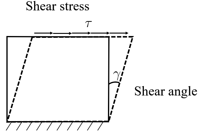
σ = E ε \boxed{\sigma =E\varepsilon} σ = Eε Given some shear stress τ \tau τ γ \gamma γ
τ = G γ \boxed{\tau = G\gamma} τ = G γ where G G G
Adding tensile deformation to the mix we get the general state of deformation on a infinitesimal element.
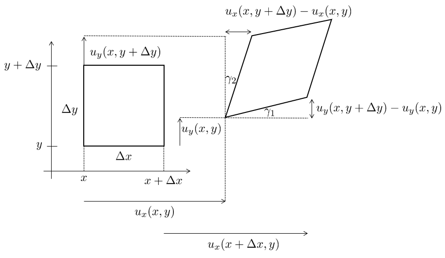
In two dimensions we will have two tensile deformations (described by u x u_x u x u y u_y u y γ 1 \gamma_1 γ 1 γ 2 \gamma_2 γ 2
The strain in the x-direction can be derived from the infinitesimal element getting displaced
u x ( x + Δ x , y ) − u x ( x , y ) Δ x → ∂ u x ∂ x = : ε x \dfrac{u_x \left(x+\Delta x,y\right)-u_x \left(x,y\right)}{\Delta x}\to \dfrac{\partial u_x }{\partial x}=:\varepsilon_x Δ x u x ( x + Δ x , y ) − u x ( x , y ) → ∂ x ∂ u x =: ε x and in the y-direction
u y ( x , y + Δ y ) − u y ( x , y ) Δ y → ∂ u y ∂ y = : ε y \dfrac{u_y \left(x,y+\Delta y\right)-u_y \left(x,y\right)}{\Delta y}\to \dfrac{\partial u_y }{\partial y}=:\varepsilon_y Δ y u y ( x , y + Δ y ) − u y ( x , y ) → ∂ y ∂ u y =: ε y The shear strain is derived by
u y ( x + Δ x , y ) − u y ( x , y ) Δ x → ∂ u y ∂ x \dfrac{u_y \left(x+\Delta x,y\right)-u_y \left(x,y\right)}{\Delta x}\to \dfrac{\partial u_y }{\partial x} Δ x u y ( x + Δ x , y ) − u y ( x , y ) → ∂ x ∂ u y Using trigonometry we can see that
tan ( γ 1 ) = u y ( x + Δ x , y ) − u y ( x , y ) Δ x → ∂ u y ∂ x \tan \left(\gamma_1 \right)=\dfrac{u_y \left(x+\Delta x,y\right)-u_y \left(x,y\right)}{\Delta x}\to \dfrac{\partial u_y }{\partial x} tan ( γ 1 ) = Δ x u y ( x + Δ x , y ) − u y ( x , y ) → ∂ x ∂ u y We assume small deformations such that we can apply the small angle approximation
tan ( γ 1 ) ≈ γ 1 \tan \left(\gamma_1 \right)\approx \gamma_1 tan ( γ 1 ) ≈ γ 1 The total shear angle is given by
γ x y = γ 1 + γ 2 \gamma_{x y} =\gamma_1 +\gamma_2 γ x y = γ 1 + γ 2 So we get the total shear strain
γ x y = ∂ u y ∂ x + ∂ u x ∂ y \gamma_{x y} =\dfrac{\partial u_y }{\partial x}+\dfrac{\partial u_x }{\partial y} γ x y = ∂ x ∂ u y + ∂ y ∂ u x This reasoning is extended into 3D such that we get
ε z = ∂ u z ∂ z , γ x z = ∂ u x ∂ z + ∂ u z ∂ x , γ y z = ∂ u y ∂ z + ∂ u z ∂ y \varepsilon_z =\dfrac{\partial u_z }{\partial z},\gamma_{x z} =\dfrac{\partial u_x }{\partial z}+\dfrac{\partial u_z }{\partial x},{ \gamma }_{y z} =\dfrac{\partial u_y }{\partial z}+\dfrac{\partial u_z }{\partial y} ε z = ∂ z ∂ u z , γ x z = ∂ z ∂ u x + ∂ x ∂ u z , γ yz = ∂ z ∂ u y + ∂ y ∂ u z In total we get six strains, which can be represented in a matrix
ε = [ ε x 1 2 γ x y 1 2 γ x z 1 2 γ x y ε y 1 2 γ y z 1 2 γ x z 1 2 γ y z ε z ] \bm \varepsilon =\left\lbrack \begin{array}{ccc}
\varepsilon_x & \dfrac{1}{2}\gamma_{x y} & \dfrac{1}{2}\gamma_{x z} \\
\dfrac{1}{2}\gamma_{x y} & \varepsilon_y & \dfrac{1}{2}\gamma_{y z} \\
\dfrac{1}{2}\gamma_{x z} & \dfrac{1}{2}\gamma_{y z} & \varepsilon_z
\end{array}\right\rbrack ε = ⎣ ⎡ ε x 2 1 γ x y 2 1 γ x z 2 1 γ x y ε y 2 1 γ yz 2 1 γ x z 2 1 γ yz ε z ⎦ ⎤ where 1 2 γ x y \frac{1}{2}\gamma_{x y} 2 1 γ x y
ε i j = 1 2 ( ∂ u i ∂ x j + ∂ u j ∂ x i ) \varepsilon_{i j} =\dfrac{1}{2}\left(\dfrac{\partial u_i }{\partial x_j }+\dfrac{\partial u_j }{\partial x_i }\right) ε ij = 2 1 ( ∂ x j ∂ u i + ∂ x i ∂ u j ) so for e.g., ε x = ε 11 = 1 2 ( ∂ u 1 ∂ x 1 + ∂ u 1 ∂ x 1 ) = ∂ u 1 ∂ x 1 = ∂ u x ∂ x \varepsilon_{x } =\varepsilon_{11} =\frac{1}{2}\left(\frac{\partial u_1 }{\partial x_1 }+\frac{\partial u_1 }{\partial x_1 }\right)=\frac{\partial u_1 }{\partial x_1 }=\frac{\partial u_x }{\partial x} ε x = ε 11 = 2 1 ( ∂ x 1 ∂ u 1 + ∂ x 1 ∂ u 1 ) = ∂ x 1 ∂ u 1 = ∂ x ∂ u x
ε x y = ε 12 = 1 2 ( ∂ u 1 ∂ x 2 + ∂ u 2 ∂ x 1 ) = ∂ u x ∂ y + ∂ u y ∂ x \varepsilon_{x y} =\varepsilon_{12} =\dfrac{1}{2}\left(\dfrac{\partial u_1 }{\partial x_2 }+\dfrac{\partial u_2 }{\partial x_1 }\right)=\dfrac{\partial u_x }{\partial y}+\dfrac{\partial u_y }{\partial x} ε x y = ε 12 = 2 1 ( ∂ x 2 ∂ u 1 + ∂ x 1 ∂ u 2 ) = ∂ y ∂ u x + ∂ x ∂ u y The stresses can be expressed in the same way
σ = [ σ x τ x y τ x z τ x y σ y τ y z τ x z τ y z σ z ] \sigma =\left\lbrack \begin{array}{ccc}
\sigma_x & \tau_{x y} & \tau_{x z} \\
\tau_{x y} & \sigma_y & \tau_{y z} \\
\tau_{x z} & \tau_{y z} & \sigma_z
\end{array}\right\rbrack σ = ⎣ ⎡ σ x τ x y τ x z τ x y σ y τ yz τ x z τ yz σ z ⎦ ⎤ Deriving the force equilibrium
On an infinitesimal element, we can assume σ y ( x , y ) \sigma_y \left(x,y\right) σ y ( x , y ) σ y ( x , y + Δ y ) \sigma_y \left(x,y+\Delta y\right) σ y ( x , y + Δ y ) x − x- x −
∑ F x = 0 ⇒ Δ σ x Δ y + Δ τ y x Δ x + f x Δ x Δ y = 0 \sum F_x =0\Rightarrow {\Delta \sigma }_x \Delta y+{\Delta \tau }_{y x} \Delta x+f_x \Delta x\Delta y=0 ∑ F x = 0 ⇒ Δ σ x Δ y + Δ τ y x Δ x + f x Δ x Δ y = 0 ⟶ : ( σ x ( x + Δ x , y ) − σ x ( x , y ) ) Δ y + ( τ y x ( x , y + Δ y ) − τ y x ( x , y ) ) Δ x + f x Δ x Δ y = 0 \longrightarrow :\left(\sigma_x \left(x+\Delta x,y\right)-\sigma_x \left(x,y\right)\right)\Delta y+\left(\tau_{y x} \left(x,y+\Delta y\right)-\tau_{y x} \left(x,y\right)\right)\Delta x+f_x \Delta x\Delta y=0 ⟶: ( σ x ( x + Δ x , y ) − σ x ( x , y ) ) Δ y + ( τ y x ( x , y + Δ y ) − τ y x ( x , y ) ) Δ x + f x Δ x Δ y = 0 and similarly for the y − y- y −
This leads to the system
− ∂ σ x ∂ x − ∂ τ y x ∂ y = f x − ∂ σ y ∂ y − ∂ τ x y ∂ x = f y \begin{array}{l}
-\dfrac{\partial \sigma_x }{\partial x}-\dfrac{\partial \tau_{y x} }{\partial y}=f_x \\
-\dfrac{\partial \sigma_y }{\partial y}-\dfrac{\partial \tau_{x y} }{\partial x}=f_y
\end{array} − ∂ x ∂ σ x − ∂ y ∂ τ y x = f x − ∂ y ∂ σ y − ∂ x ∂ τ x y = f y This can be expressed using matrix notation
− ∂ ∂ x [ σ x τ x y ] − ∂ ∂ y [ τ x y σ x ] = [ f x f y ] -\dfrac{\partial }{\partial x}\left\lbrack \begin{array}{c}
\sigma_x \\
\tau_{x y}
\end{array}\right\rbrack -\dfrac{\partial }{\partial y}\left\lbrack \begin{array}{c}
\tau_{x y} \\
\sigma_x
\end{array}\right\rbrack =\left\lbrack \begin{array}{c}
f_x \\
f_y
\end{array}\right\rbrack − ∂ x ∂ [ σ x τ x y ] − ∂ y ∂ [ τ x y σ x ] = [ f x f y ] Recall the gradient operator ∇ \nabla ∇
∇ = [ ∂ ∂ x ∂ ∂ y ] \nabla =\left\lbrack \begin{array}{c}
\dfrac{\partial }{\partial x}\\
\dfrac{\partial }{\partial y}
\end{array}\right\rbrack ∇ = ⎣ ⎡ ∂ x ∂ ∂ y ∂ ⎦ ⎤ The divergence of the stress matrix is
− ∇ ⋅ σ = f = − ∂ ∂ x [ σ x τ x y ] − ∂ ∂ y [ τ x y σ x ] = [ f x f y ] -\nabla \cdot \sigma =f=-\dfrac{\partial }{\partial x}\left\lbrack \begin{array}{c}
\sigma_x \\
\tau_{x y}
\end{array}\right\rbrack -\dfrac{\partial }{\partial y}\left\lbrack \begin{array}{c}
\tau_{x y} \\
\sigma_x
\end{array}\right\rbrack =\left\lbrack \begin{array}{c}
f_x \\
f_y
\end{array}\right\rbrack − ∇ ⋅ σ = f = − ∂ x ∂ [ σ x τ x y ] − ∂ y ∂ [ τ x y σ x ] = [ f x f y ] Thus the short hand notation for the equilibrium equation using tensor notation is
− ∇ ⋅ σ = f \boxed{-\nabla \cdot \bm \sigma = \bm f} − ∇ ⋅ σ = f A moment equilibrium around the midpoint gives:
τ x y ( x + Δ x , y ) Δ y 1 2 Δ x + τ x y ( x , y ) Δ y 1 2 Δ x − τ y x ( x , y ) Δ x 1 2 Δ y − τ y x ( x , y + Δ y ) Δ x 1 2 Δ y = 0 \tau_{x y} \left(x+\Delta x,y\right)\Delta y \dfrac{1}{2} \Delta x+\tau_{x y} \left(x,y\right)\Delta y \dfrac{1}{2} \Delta x-\tau_{y x} \left(x,y\right)\Delta x\dfrac{1}{2}\Delta y-\tau_{y x} \left(x,y+\Delta y\right)\Delta x \dfrac{1}{2} \Delta y=0 τ x y ( x + Δ x , y ) Δ y 2 1 Δ x + τ x y ( x , y ) Δ y 2 1 Δ x − τ y x ( x , y ) Δ x 2 1 Δ y − τ y x ( x , y + Δ y ) Δ x 2 1 Δ y = 0 This simplifies to
⇒ τ x y ( x + Δ x , y ) + τ x y ( x , y ) = τ y x ( x , y + Δ y ) + τ y x ( x , y ) \Rightarrow \tau_{x y} \left(x+\Delta x,y\right)+\tau_{x y} \left(x,y\right)=\tau_{y x} \left(x,y+\Delta y\right)+\tau_{y x} \left(x,y\right) ⇒ τ x y ( x + Δ x , y ) + τ x y ( x , y ) = τ y x ( x , y + Δ y ) + τ y x ( x , y ) with Δ x → 0 \Delta x\to 0 Δ x → 0 Δ y → 0 \Delta y\to 0 Δ y → 0
we have τ x y = τ y x \tau_{xy} =\tau_{yx} τ x y = τ y x τ y z = τ z y \tau_{y z} =\tau_{z y} τ yz = τ zy τ x z = τ z x \tau_{x z} =\tau_{z x} τ x z = τ z x
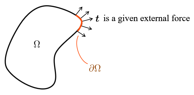
On a deformable body Ω \Omega Ω t t t ∂ Ω \partial \Omega ∂ Ω
The external force t t t
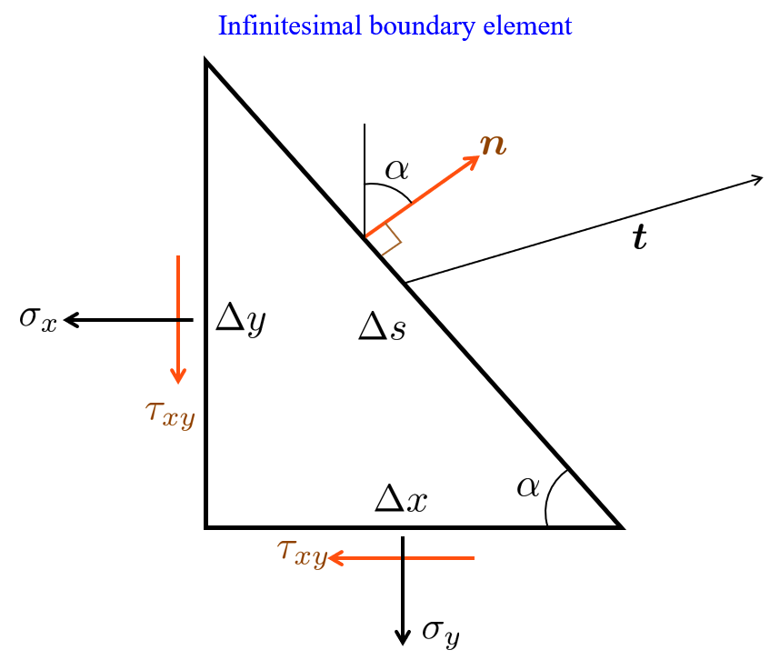
On an infinitesimal boundary element the boundary can be said to be a small straight line, Δ s \Delta s Δ s α \alpha α
From the figure we can establish the following kinematic relations
Δ s = Δ x 2 + Δ y 2 Δ x = cos α Δ s Δ y = sin α Δ s \begin{array}{l}
\Delta s=\sqrt{\Delta x^2 +\Delta y^2 }\\
\Delta x=\cos \alpha \Delta s\\
\Delta y=\sin \alpha \Delta s
\end{array} Δ s = Δ x 2 + Δ y 2 Δ x = cos α Δ s Δ y = sin α Δ s n = [ sin α , cos α ] \bm n=\left\lbrack \sin \alpha ,\cos \alpha \right\rbrack n = [ sin α , cos α ] Equilibrium gives:
⟵ : σ x Δ y + τ x y Δ x = t x Δ s = σ x sin α + τ x y cos α = t x ↓ : σ x Δ x + τ x y Δ y = t y Δ s = σ x cos α + τ x y sin α = t y \begin{array}{l}
\longleftarrow :\sigma_x \Delta y+\tau_{x y} \Delta x=t_x \Delta s=\sigma_x \sin \alpha +\tau_{x y} \cos \alpha =t_x \\
\downarrow :\sigma_x \Delta x+\tau_{x y} \Delta y=t_y \Delta s=\sigma_x \cos \alpha +\tau_{x y} \sin \alpha =t_y
\end{array} ⟵: σ x Δ y + τ x y Δ x = t x Δ s = σ x sin α + τ x y cos α = t x ↓: σ x Δ x + τ x y Δ y = t y Δ s = σ x cos α + τ x y sin α = t y ⇒ σ x n x + τ x y n y = t x σ x n y + τ x y n y = t n } [ σ x τ x y τ x y σ y ] [ n x n y ] = [ t x t y ] \left.\Rightarrow \begin{array}{c}
\sigma_x n_x +\tau_{x y} n_y =t_x \\
\sigma_x n_y +\tau_{x y} n_y =t_n
\end{array}\right\rbrace \left\lbrack \begin{array}{cc}
\sigma_x & \tau_{x y} \\
\tau_{x y} & \sigma_y
\end{array}\right\rbrack \left\lbrack \begin{array}{c}
n_x \\
n_y
\end{array}\right\rbrack =\left\lbrack \begin{array}{c}
t_x \\
t_y
\end{array}\right\rbrack ⇒ σ x n x + τ x y n y = t x σ x n y + τ x y n y = t n } [ σ x τ x y τ x y σ y ] [ n x n y ] = [ t x t y ] or
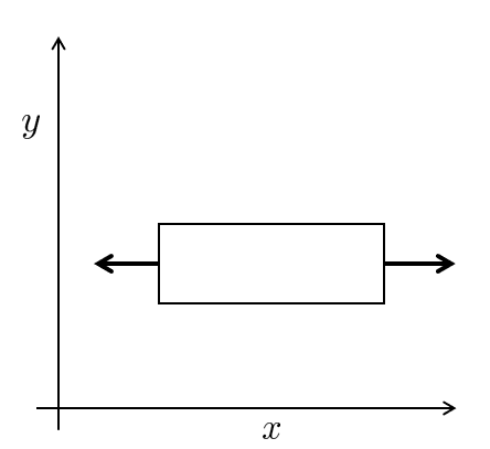
σ ⋅ n = t \boxed{\bm\sigma \cdot \bm n = \bm t} σ ⋅ n = t A 2D geometry in pure tension along the x-axis experiences mostly stress in the x-direction and some amount of transversal contraction stress in the y-direction, but no shear stress.
σ = [ σ x τ x y τ x y σ y ] = [ σ x 0 0 σ y ] \sigma =\left\lbrack \begin{array}{cc}
\sigma_x & \tau_{x y} \\
\tau_{x y} & \sigma_y
\end{array}\right\rbrack =\left\lbrack \begin{array}{cc}
\sigma_x & 0\\
0 & \sigma_y
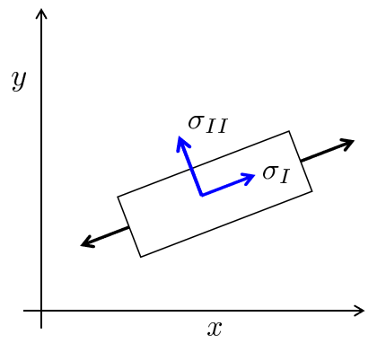
\end{array}\right\rbrack σ = [ σ x τ x y τ x y σ y ] = [ σ x 0 0 σ y ] If we apply the same load case to the geometry but rotate the frame of reference than we will get shear stress since our matrix is expressed in terms of the x and y coordinates and not the local body coordinates.
σ = [ σ x τ x y τ x y σ y ] = [ σ x ≠ 0 τ x y ≠ 0 τ x y ≠ 0 σ y ≠ 0 ] \sigma =\left\lbrack \begin{array}{cc}
\sigma_x & \tau_{x y} \\
\tau_{x y} & \sigma_y
\end{array}\right\rbrack =\left\lbrack \begin{array}{cc}
\sigma_x \not= 0 & \tau_{x y} \not= 0\\
\tau_{x y} \not= 0 & \sigma_y \not= 0
\end{array}\right\rbrack σ = [ σ x τ x y τ x y σ y ] = [ σ x = 0 τ x y = 0 τ x y = 0 σ y = 0 ] Computing these "local coordinate stresses" is important since it gives us an understanding if the stress is in tension or compression. This change of reference system such that we get rid of the shear stress is called Principal stress .
If the traction is normal to the surface, then we can write
t = λ n t=\lambda n t = λn where λ \lambda λ
σ ⋅ n = t ⇒ σ ⋅ n = λ n \sigma \cdot \mathit{\mathbf{n} }=t\Rightarrow \sigma \cdot \mathit{\mathbf{n} }=\lambda \mathit{\mathbf{n} } σ ⋅ n = t ⇒ σ ⋅ n = λ n or
( σ − λ I ) ⋅ n = 0 \left(\sigma -\lambda I\right)\cdot \mathit{\mathbf{n} }=0 ( σ − λ I ) ⋅ n = 0 This is an eigenvalue problem
We can find non-zero solutions by solving
det ( σ − λ I ) = 0 \det \left(\sigma -\lambda I\right)=0 det ( σ − λ I ) = 0 ∣ σ x − λ σ x y σ x y σ y − λ ∣ = ( σ x − λ ) ( σ y − λ ) − σ x y 2 = 0 \left|\begin{array}{cc}
\sigma_x -\lambda & \sigma_{x y} \\
\sigma_{x y} & \sigma_y -\lambda
\end{array}\right|=\left(\sigma_x -\lambda \right)\left(\sigma_y -\lambda \right)-{\sigma_{x y} }^2 =0 ∣ ∣ σ x − λ σ x y σ x y σ y − λ ∣ ∣ = ( σ x − λ ) ( σ y − λ ) − σ x y 2 = 0 λ 2 − ( σ x + σ y ) ⏟ t r a c e ( σ ) λ + σ x σ y − σ x y 2 ⏟ det ( σ ) = 0 \lambda^2 -\underset{\mathrm{trace}\left(\sigma \right)}{\underbrace{\left(\sigma_x +\sigma_y \right)} } \lambda +\underset{\det \left(\sigma \right)}{\underbrace{\sigma_x \sigma_y -{\sigma_{x y} }^2 } } =0 λ 2 − trace ( σ ) ( σ x + σ y ) λ + d e t ( σ ) σ x σ y − σ x y 2 = 0 The roots to this equation, λ I \lambda_I λ I λ I I \lambda_{\mathrm{II} } λ II
Using the principal stresses in a general 3D stress state, σ 1 , σ 2 , σ 3 \sigma_1 ,\sigma_2 ,\sigma_3 σ 1 , σ 2 , σ 3
σ v M = 1 2 [ ( σ 1 − σ 2 ) 2 + ( σ 2 − σ 3 ) 2 + ( σ 3 − σ 1 ) 2 ] \sigma_{\mathrm{vM} } =\sqrt{\dfrac{1}{2}\left\lbrack {\left(\sigma_1 -\sigma_2 \right)}^2 +{\left(\sigma_2 -\sigma_3 \right)}^2 +{\left(\sigma_3 -\sigma_1 \right)}^2 \right\rbrack } σ vM = 2 1 [ ( σ 1 − σ 2 ) 2 + ( σ 2 − σ 3 ) 2 + ( σ 3 − σ 1 ) 2 ] or using the general 3D stress components
σ v M = 1 2 [ ( σ x − σ y ) 2 + ( σ y − σ z ) 2 + ( σ z − σ x ) 2 + 6 ( σ x y 2 + σ y z 2 + σ z x 2 ) ] \sigma_{\mathrm{vM} } =\sqrt{\dfrac{1}{2}\left\lbrack {\left(\sigma_x -\sigma_y \right)}^2 +{\left(\sigma_y -\sigma_z \right)}^2 +{\left(\sigma_z -\sigma_x \right)}^2 +6\left({\sigma_{x y} }^2 +{\sigma_{y z} }^2 +{\sigma_{z x} }^2 \right)\right\rbrack } σ vM = 2 1 [ ( σ x − σ y ) 2 + ( σ y − σ z ) 2 + ( σ z − σ x ) 2 + 6 ( σ x y 2 + σ yz 2 + σ z x 2 ) ] For general plane stress (2D) this simplifies since σ z = σ y z = σ z x = 0 \sigma_z =\sigma_{y z} =\sigma_{z x} =0 σ z = σ yz = σ z x = 0
σ v M = σ x 2 − σ x σ y + σ y 2 + 3 σ x y 2 \sigma_{\mathrm{vM} } =\sqrt{ {\sigma_x }^2 -\sigma_x \sigma_y +{\sigma_y }^2 +3{\sigma_{x y} }^2 } σ vM = σ x 2 − σ x σ y + σ y 2 + 3 σ x y 2 More info on the failure theories is given by the efficient engineer .