Applied Mechanics

Table of contents

Video Lecture (swedish)

Intro to equilibrium

Equilibrium part 2

Static Equilibrium (Statisk jämvikt)

Statics

$$\begin{array}{l} \sum \mathit{\mathbf{F} }=0\\ \sum \mathit{\mathbf{M} }=0 \end{array}$$

Solution strategy

1. What is known and unknown?

2. Free body diagram

3. Insert coordinate system

4. Identify a suitable point for a moment equation.

5. $\displaystyle \Sigma \mathit{\mathbf{M} }=0$

6. $\displaystyle \Sigma \mathit{\mathbf{F} }=0$

7. Solve the equation system for the unknowns

8. Analyze the results, plot, visualize

9. Conclusion

Example 1

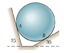
A sphere with a mass $m$ is resting against smooth surfaces according to the figure above. Determine the normal force at $A$ and $B$.

Solution

Welcome to the swamp of angles (vinkelträsket)! Insert a Cartesian coordinate system i the center of the sphere and create a free body diagram for the sphere!

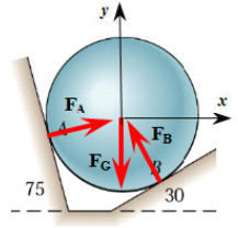
Since the surfaces are smooth they can only give rise to normal forces. We thus have contact forces at $A$ and $B$, as well as a weight force which acts on the center of the sphere. Since all forces are directed through the center of the sphere, force equilibrium will be enough to solve for all unknowns.

$$\sum_{\;} {\mathit{\mathbf{F} } }_i =0$$

clear
syms F_A F_B m g

We can handle the swamp of angles in a systematic way. Define the angles from the $x$-axis ($\left\lbrack 1,0\right\rbrack$) positively counter-clockwise.

We can thus create a unit vector as a function of the angle $\theta$:

$$\mathit{\mathbf{e} }\left(\theta \right):=\left\lbrack \cos \left(\theta \right),\sin \left(\theta \right),0\right\rbrack^T$$

In Matlab, this can be done using an e.g., an anonymous function:

e = @(theta)[cosd(theta); sind(theta); 0];

Now we can get the direction of ${\mathit{\mathbf{F} } }_A$ by starting at ${180}^{\circ }$ and rotating "backwards" ${75}^{\circ }$ and then again ${90}^{\circ }$ to point in the direction we see in the figure.

FFA = F_A*e(180-75-90)

Matlab sometimes cannot simplify expressions other than approximating it with a fraction. This is accurate but not readable, for this reason we can display the answer as a decimal number with an arbitrary precision, here we choose two significant numbers.

vpa(FFA,2)

Then we have ${\mathit{\mathbf{F} } }_B$:

FFB = F_B*e(30+90)

vpa(FFB,2)

The weight vector is simply

FG = [0;-m*g;0]

Equilibrium stated that:

ekv = FFA+FFB+FG == 0;

The above expression is exact, but hard to read, so we display the decimal form of it using vpa and then we can analyze the equation system.

vpa(ekv,2)

Now we can send the equation to the solver and solve for $F_B$ and $F_A$.

[F_A,F_B] = solve(ekv,[F_A,F_B]);

We simplify the expression

F_A = vpa(simplify(F_A),2)

F_B = vpa(simplify(F_B),2)

$F_B$ is simplified to $mg$!

The conclusion is that $F_B$ takes the whole wight while $F_A$ only takes about half of the spheres weight. This seems reasonable judging from the figure and FBD.

For a complete analysis we can rotate the whole system ${30}^{\circ }$ clockwise such that $F_B$ is pointing straight up and $F_A$ thus is zero. Try it to confirm.

Example 2

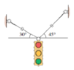
Determine the wire tensions which carry the traffic light. The light has a mass of $m$kg.

Solution

Insert a coordinate system and create a FBD.

We'll use the same approach as in example 2. Define the angles from the $x$-axis ($\left\lbrack 1,0\right\rbrack$) positively counter-clockwise.

clear
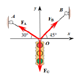
e = @(theta)[cosd(theta); sind(theta); 0];

Similarly to example 2, since all forces are acting through the Origin, a force equilibrium is enough to determine the unknowns.

syms FA FB mg
FFA = FA*e(180-30); vpa(FFA,2)

FFB = FB*e(45); vpa(FFB,2)

FG = [0;-mg;0];

ekv = FFA+FFB+FG==0; vpa(ekv,2)

[FA, FB] = solve(ekv,[FA,FB]);
FA = simplify(FA)

FB = simplify(FB)

vpa(FA,2)

vpa(FB,2)

Conclusion: $F_B$ is bigger than $F_A$ because the point B is higher. If both angles had been ${30}^{\circ }$ then the wire forces would have been the same and equal to $m\;g$.

Example 3

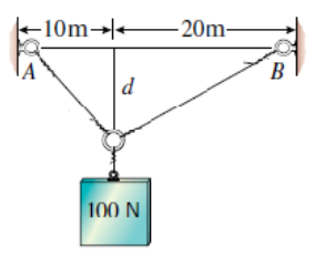
Determine the wire tensions as a function of the distance $d$. Plot both forces and analyze the results!

Solution

In contrast to the previous two academic examples, forces in real life are typically always going along a line of action and are defined from one point to another. In this example, we have forces along a line which is hung up between three points.

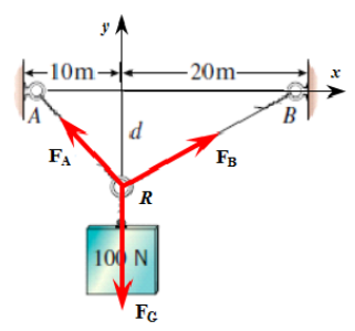
We start by inserting a coordinate system according to the FBD. Then positional vectors.

$$\overrightarrow{\textrm{OA} } ={\left\lbrack -10,0,0\right\rbrack }^T ,\overrightarrow{\textrm{OB} } ={\left\lbrack 20,0,0\right\rbrack }^T ,\overrightarrow{\textrm{OR} } ={\left\lbrack 0,-d,0\right\rbrack }^T$$

clear
syms d positive

We create a variable $d$ and set it to be positive, this will simplify the expressions. See for yourself, try and experiment!

OA = [-10, 0, 0].'; OB = [20, 0, 0].'; OR = [0, -d, 0].';

Then wire forces which act from point $R$ toward points $A$ and $B$.

syms v FA FB
RA = OA-OR;
RB = OB-OR;
FFA = FA*RA/norm(RA)

FFB = FB*RB/norm(RB)

FG = [0; -100; 0];

ekv = [FFA+FFB+FG==0]

[FA, FB] = solve(ekv, [FA, FB])

figure; hold on
fplot(FA,[1,20],'Color','r','LineWidth',2,'DisplayName','F_A')
fplot(FB,[1,20],'Color','b','LineWidth',2,'DisplayName','F_B')
legend
ylim([0,200])

Here we can see that the wire forces are tending towards infinity as $d\to 0$. This is intuitive. Again, we can set the distances such that the weight hangs symmetrically and check the feasibility of our model.

We end with a limit as $d\to \infty$.

vpa(limit([FA,FB],d,inf),3)

Conclusion: $F_A \to 66\ldotp 7\mathrm{N}$ and $F_B \to 33\ldotp 3\mathrm{N}$ with large values for $d$.

Example 4

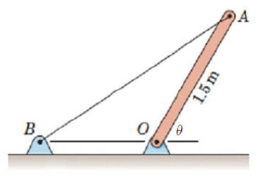
Determine the wire force and the reaction forces in the Origin if the homogeneous rod has a mass of $m$ kg and is free to rotate at $O$.

Solution

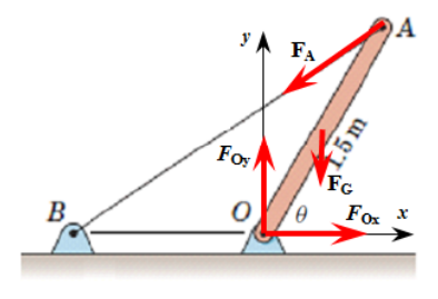
Insert a coordinate system and positional vectors to all important points. Use the defined points to describe new points. We want to vary the position of $B$ along the $x$-axis as well as the slope, $\theta$ of the rod.

clear
syms theta b
e = @(theta)[cosd(theta),sind(theta),0].';
OA = 1.5*e(theta);
OB = [-b, 0, 0].';
OG = OA/2;

Now, the forces, start with the wire force.

syms F_A
AB = OB-OA;
FFA = F_A*AB/norm(AB)

Weight force

syms mg
FG = [0, -mg, 0].';

Reaction force in O.

syms R_x R_y
FO = [R_x, R_y, 0].';

Equilibrium

We have $\sum_{\;} \mathit{\mathbf{F} }=0$ and $\sum_{\;} M_O =0$.

ekv = [FFA+FG+FO==0;
       cross(OA,FFA)+cross(OG,FG)==0]

As we can see, we always get 6 equations and in 2D we always have three real equations, $\Sigma F_x =0,\Sigma F_y =0,\Sigma M_z =0$.

We have three equations and three unknown variables: $R_x ,R_y \;\&\;F_A$

Solve the system of equations

[R_x, R_y, F_A] = solve(ekv,[R_x, R_y, F_A] )

Analysis

The resulting expressions are hard to make sense of! We need to plot!

We will set $\theta =60\degree$ and vary $b$. Then we'll set $b=1\ldotp 5$ and vary $\theta$.

Visualize stuff as much as possible, the eye is excellent at discovering interesting things!

mg = 1; theta = 60;
figure; hold on;
fplot(subs(F_A),[0.25,2],'Displayname','F_A(\theta=60^\circ)')
fplot(subs(R_x),[0.25,2],'Displayname','R_x(\theta=60^\circ)')
fplot(subs(R_y),[0.25,2],'Displayname','R_y(\theta=60^\circ)')
legend; xlabel('b'); ylabel('F/mg');

It makes sense that all forces are tending towards infinity as $B$ tends towards the Origin.

mg = 1; b = 1.5; syms theta
figure; hold on;
fplot(subs(F_A),[0, 90],'Displayname','F_A(b=1.5)')
fplot(subs(R_x),[0, 90],'Displayname','R_x(b=1.5)')
fplot(subs(R_y),[0, 90],'Displayname','R_y(b=1.5)')
legend; xlabel('\theta'); ylabel('F/mg');
axis([0,90,0,5])

ax = gca;
chart = ax.Children(1);
datatip(chart,90,1);

As $\theta$ approached $90\degree$ the rod is vertical and all the weight is directly above the support, thus the weight vector and reaction vector cancel out, no force is acting in the horizontal direction and the wire force is thus zero. Makes perfect sense.

Example 5

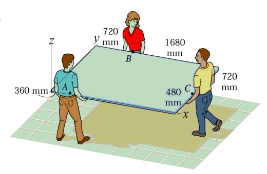
A rectangular board with a mass of $m$kg is carried in a horizontal position according to the figure above.

Create a FBD of the board, the people only exsert a force in the positive z-direction. Determine how much each person is lifting and which one of them is lifting in the least. Do you even lift bro?

Solution

Start the usual way, add a coordinate system and forces, create a FBD.

clear
OA = [0.360, 0, 0].'; OB = [0.720, 0.480+0.720, 0].';
OC = [0.720+1.680, 0.480, 0].'; OG = [0.720+1.680, 0.480+0.720,0].'/2;

The forces

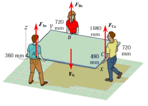
syms FAz FBz FCz mg
FA = [0, 0, FAz].'; FB = [0,0,FBz].'; FC = [0,0,FCz].'; FG = [0,0,-mg].';

Equilibrium.

$$\Sigma \mathit{\mathbf{F} }={\mathit{\mathbf{F} } }_A +{\mathit{\mathbf{F} } }_B +{\mathit{\mathbf{F} } }_C +{\mathit{\mathbf{F} } }_G$$

Let's do a moment equation around the Origin.

$$\Sigma M_O =\overrightarrow{\textrm{OA} } \times {\mathit{\mathbf{F} } }_A +\overrightarrow{\textrm{OB} } \times {\mathit{\mathbf{F} } }_B +\overrightarrow{\textrm{OC} } \times {\mathit{\mathbf{F} } }_C +\overrightarrow{\textrm{OG} } \times {\mathit{\mathbf{F} } }_G$$

ekv = [FA+FB+FC+FG;... 
       cross(OA,FA)+cross(OB,FB)+cross(OC,FC)+cross(OG,FG)]==0

[FAz, FBz, FCz] = solve(ekv, [FAz, FBz, FCz]);
vpa([FAz, FBz, FCz],3)

Feasibility, sanity check

sum([FAz, FBz, FCz])

Conclusion: The dude in A is lifting the least.

Example 6

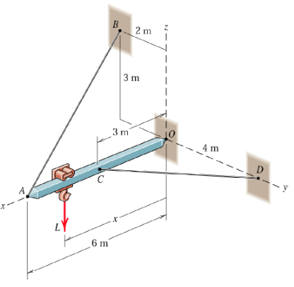
A light crane as rigged according to the figure above. Determine, as a function of $x$, the reaction forces in the $x$-direction an the two wire forces. The crane is free to rotate about the Origin. The hook-carriage can travel along the x-axis.

Determine the minimum value of $F_O /F_L$ where $F_O$ is the magnitude of the reaction force in $O$ and $F_L$ is the magnitude of the load at the carriage.

Solution

$$\Sigma \mathit{\mathbf{F} }=0$$ $$\Sigma M_O =0$$

FBD with a inserted coordinate system and forces.

clear
OA = [6,0,0].'; OB = [0, -2, 3].'; OC = [3, 0, 0].';
OD = [0, 4, 0].'; 
syms x real positive
OL = [x, 0, 0].';

Force vectors in $O$, wires, etc.

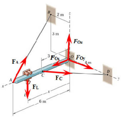
syms F_L positive real
syms FA FC FOx FOy FOz
AB = OB-OA;
CD = OD-OC;
FFA = FA*AB/norm(AB)

FFC = FC*CD/norm(CD)

FFO = [FOx, FOy, FOz].';
FFL = [0, 0, -F_L].';

Set up the force and moment equations and solve for the unknowns.

ekv = [FFA+FFC+FFO+F_L;
       cross(OA,FFA)+cross(OL,FFL)+cross(OC,FFC)]==0

[FA, FC, FOx, FOy, FOz] = solve(ekv, [FA, FC, FOx, FOy, FOz])

Finally we compute $F_O /F_L$. Studying a model of a moving load, e.g., a car that drives over a bridge, is very common for engineers. The picture of various loads as a function of the loads position is called the influence line diagram. Here is such a diagram

FO = simplify(subs(norm(FFO)))

kvot = simplify(FO/F_L)

figure
fplot(kvot, [0,2])
xlabel('x'); ylabel('F_O/F_L')

The minimum can be read from the graph or calculated with a bit of calculus:

x_min = vpa(solve(diff(kvot,x)==0,x),3)

FO_min = vpa(subs(kvot,x,x_min),3)

The resulting force in the $x$-direction is given by

FOx