Table of contents

Newtonian physics
Example 1 - Typical types of forces
Example 2
1. Solution
2. Discussion
Example 3 - Force projection
1. Solution
  1. Projection
Example 4 - normal coordinates
1. Solution
Example 5 - Solving equations
1. Solution

Newtonian physics

We begin our journey in mechanics using Newtonian physics, which works quite well in statics. Newton's model of how bodies are interacting with one another can be described by three laws

Newton's first law: The law of inertia (tröghetslagen)

A body is at rest or moving at a constant speed in a straight line unless acted upon by a force. For a body to be at rest or constant speed the forces acting on it must be in balance. This means that bodies are coming to a rest only by some friction or air resistance acting on them.

Newton's second law: The law of acceleration $F=m a$

The rate change of the momentum (rörelsemängd) of a body is equal to the force acting on it.

m\ddot{x} =F

Here we use Newton's notation for time derivatives. Using Leibniz notation, Newton's second law states

F=\dfrac{d}{dt}\left(mv\right)=m\dfrac{dv}{dt}=ma

Newton's third law: The law of action and reaction

When two bodies interact, they apply forces to one another that are equal in magnitude and opposite in direction.

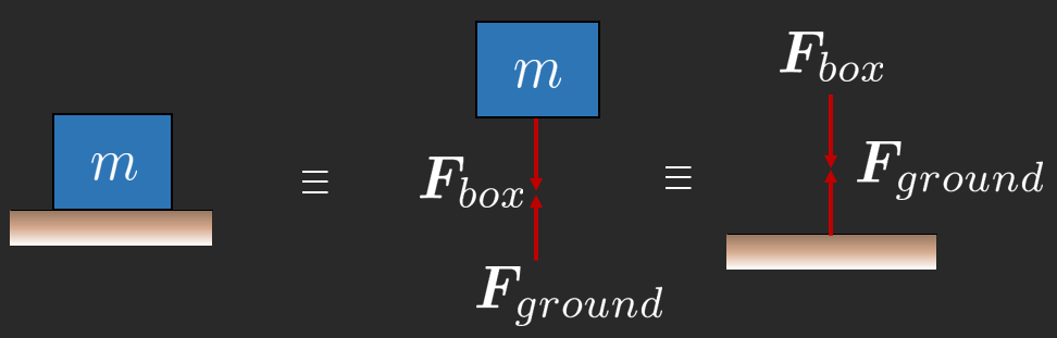
A special case is gravity, where according to Newtonian physics, two bodies are attracting each other with a force

F=G\;\dfrac{m_1 \;m_2 }{r^2 }

where $r$ is the distance between the center of masses of the two bodies and $G=6\ldotp 67\times {10}^{-11} \;{\mathrm{m} }^3 /\left(\textrm{kg}\times {\mathrm{s} }^2 \right)$ is the universal gravity constant. Setting the mass of the earth to $m_1 =5\ldotp 98\times {10}^{24} \;\textrm{kg}$ and the radius $r=6378\times {10}^3 \;\mathrm{m}$ , assuming that we are at the height $h$ over the surface of the earth, the distance between the center of the earth and an object can be assumed to be $r$ since $r>>h$ , we thus get

\mathbf F = G\;\dfrac{m_1 \;m_2 }{r^2 }=6\ldotp 67\times {10}^{-11} \;\dfrac{5\ldotp 98\times {10}^{24} \;m_2 }{ {\left(6378\times {10}^3 \right)}^2 }\;\textrm{kg}\times \mathrm{m}/{\mathrm{s} }^2 =9\ldotp 81\;m_2 \;\mathrm{N}=m_2 \;g\;\mathrm{N}

The force $\mathbf F=m_2 g$ is called the weight (tyngden) of $m_2$ , or the gravity (tyngdkraften) acting on $m_2$ which is a force vector with a unit of Newton $\left\lbrack \mathrm{N}\right\rbrack$ . Note the difference between the weight and the mass which is a scalar with the unit $\left\lbrack \textrm{kg}\right\rbrack$ .

Forces

A force is a vector, carrying information about the magnitude and direction of how a body is interacting with it's surrounding. A force can be a weight, caused by an object having a mass and being attracted by the earth, the moon or really any other object. Another type of force is a spring which has a spring force which is proportional to the springs displacement by a spring constant. We have contact forces between bodies.

A weight is continuously distributed across a bodies volume, but we model it as a total force acting at a singular point, the center of gravity of a body. The pressure acting on a balloon is distributed force across a surface. We will be dealing with both types of forces, and need to be able to go from one to another by replacing a distributed force with a point load and a point of action.

Most things in mechanics are treated as vectors, e.g., forces, torques (moments), "points of action", positions, moment arm, displacement, velocity.

We usually denote vectors with lower case bold symbols, and their scalars with the same lower case symbols. Their relationship is

a = |\underline{a}| = |\mathbf{a}|:=\sqrt{\mathbf{a}\cdot \mathbf{a} }\overset{3D}{=} \sqrt{a_x^2 +a_y^2 +a_z^2 }

The underline notation is used when writing on the board during a lecture.

A vector can be expressed in two ways

Component form: $\mathbf{a} ={\left(a_x ,a_y ,a_z \right)}^T =a_x {\mathbf{i} }+a_y \mathbf{j}+a_z \mathbf{k}$ where the later is a linear combination of standard bases (Cartesian base vectors) and the components. We always denote vectors as column vectors. For convenance and to save space we write them as row-vectors and transpose them. Points are the exception, they are written out as row vectors e.g., $A=\left(1,2,4\right)$ .

Vector form (pointing): $\mathbf{a} =| \mathbf{a} |\mathbf{e}_a$ , where $\mathbf{e}_\mathbf{a}$ is a unit vector (a vector of unit length) pointing in a:s direction.

In mechanics we tend to break the naming convention and use capital letters to denote forces, torques and points. e.g., $\mathit{\mathbf{F} }=F\;{\mathit{\mathbf{e} } }_F$ .

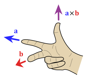
Note the difference between a point and a position vector. A point can be e.g., $A=\left(1,2,1\right)$ but a position vector is a vector defined as starting in the origin and ending in the point, e.g., ${\mathit{\mathbf{r} } }_A =\overrightarrow{\textrm{OA} } ={\left(1,2,1\right)}^T$

Using the right-hand rule we define a coordinate system with $x$ positively to the right, $y$ positively up and thus $z$ is given positively outward from the screen.

We will see many problems that are simplified into 2D, so called plane problems, these are remnants of the old days when we only could do calculations by hand. With modern computer tools we can treat vectors naturally as 3D vectors, with the additional advantage of being able to visualize them. However, many problems can still be accurately simplified into 2D.

The cursed angles

Be vary of introducing angles for computation! Only accept angles as input data (with skepticism) to create a proper vector. Angles occur naturally to parameterize kinematics, this is not a case where we want to avoid angles. What we mean is situations where angles are introduced to formulate directions without there being an explicit need. See example 1 below for an example.

Example 1 - Typical types of forces

These are the most typical types of forces that can appear in the wild.

We shall define these as vectors. $\mathbf{F}_1 =600\left(\cos \;35\degree ,\sin \;35\degree ,0\right)$ , ${\mathit{\mathbf{F} } }_2 =500\left(-\frac{4}{5},\frac{3}{5},0\right)$

For $\mathbf F_2$ we could have introduced an angle, but this is not necessary and should be avoided!

The last force is closer to how a force would be described outside of a textbook on mechanics, in the real world: a force in a point acting towards another point. This is much easier to measure in the real world.

{\mathit{\mathbf{F} } }_3 =800\;{\mathit{\mathbf{e} } }_{\overrightarrow{\textrm{AB} } } =800\;\dfrac{\overrightarrow{\textrm{AB} } }{|\overrightarrow{\textrm{AB} } |}\;

clear
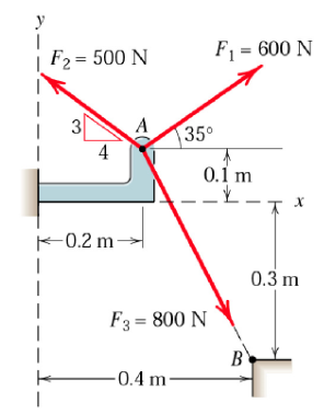
F1 = 600*[cosd(35), sind(35), 0].'

F2 = 500*[-4/5, 3/5, 0].'

In Matlab we can quickly compute the norm (magnitude) of a vector simply by using the function norm() which basically does $\sqrt{\mathit{\mathbf{a} }\cdot \mathit{\mathbf{a} } }$ .

Many times we need to compute the unit vector for some vector $\mathit{\mathbf{a} }$ . Unfortunately there is no built in function in Matlab to do so. But we can create our own functions easily, the simplest way is to create an anonymous function.

normalize = @(a)a./norm(a);

No we can easily create that third vector.

{\mathit{\mathbf{F} } }_3 =800\;\dfrac{\overrightarrow{\textrm{OB} } -\overrightarrow{\textrm{OA} } }{|\overrightarrow{\textrm{OB} } -\overrightarrow{\textrm{OA} } |}

F3 = 800*normalize([0.4,-0.3,0] - [0.2, 0.1, 0]).'

The resulting force, $\mathit{\mathbf{R} }=\sum {\mathit{\mathbf{F} } }_i = {\mathit{\mathbf{F} } }_1 +{\mathit{\mathbf{F} } }_2 +{\mathit{\mathbf{F} } }_3$

R = F1+F2+F3

And its magnitude, $R=|\mathit{\mathbf{R} }|$

norm(R)

ans = 454.8998

In practice, for dimensioning purposes, both the resulting force and the components of forces are of interest. In this case we might be interested in the resulting force in the y-direction, which we can get directly by reading the vector or accessing (indexing) the vector.

R(2)

ans = -71.3959

Finally, we plot the situation.

figure
OA = [0.2,0.1,0]';
OB = [0.4,-0.3,0]';
plot([OA(1),OB(1)],[OA(2),OB(2)],'k--','HandleVisibility','off');
hold on; axis equal;
axis([0,0.5,-0.4,0.3])
quiver(OA(1),OA(2),F1(1),F1(2),0.2/norm(F1),'b','LineWidth',2,'Displayname','F1')
quiver(OA(1),OA(2),F2(1),F2(2),0.2/norm(F2),'c','LineWidth',2,'Displayname','F2')
quiver(OA(1),OA(2),F3(1),F3(2),0.2/norm(F3),'r','LineWidth',2,'Displayname','F3')
quiver(OA(1),OA(2),R(1),R(2),0.2/norm(R),'k','LineWidth',2,'Displayname','R')
legend('show','Location','southwest')

Example 2

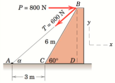
Combine the two forces $\mathit{\mathbf{P} }\;\textrm{and}\;\mathit{\mathbf{T} }$ , which act on the fixed structure at B, into a single equivalent force $\mathit{\mathbf{R} }\ldotp$

Solution

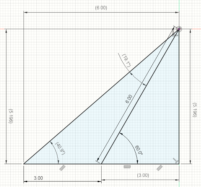
Set the origin in the point $B$ and compute $\overrightarrow{\textrm{OA} }$ .

The height is $\textrm{BD}=6 \sin \left({60}^{\circ } \right)$

\text{CD} = 6 \cos(60^\circ)

\overrightarrow{OA} = [-(3+CD),-BD,0]^T

\boldsymbol T = 600 \dfrac{\overrightarrow{OA}}{|\overrightarrow{OA}|}

\boldsymbol R = \boldsymbol T + \boldsymbol P

clear
normalize = @(a)a./norm(a);

BD = 6*sind(60)

BD = 5.1962

CD = 6*cosd(60)

CD = 3

OA = [-(3+CD),-BD,0]'

T = 600*normalize(OA)

P = [800,0,0]'

R = T+P

norm(R)

ans = 523.7444

Discussion

You can verify the geometry using a simple CAD sketch, see the figure below.

1: Fusion 360 sketch.

Example 3 - Force projection

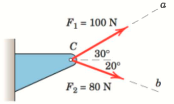
Forces ${\mathit{\mathbf{F} } }_1$ and ${\mathit{\mathbf{F} } }_2 \;\;$ act on the bracket as shown. Determine the projection ${\mathit{\mathbf{F} } }_b$ of their resultant $\mathit{\mathbf{R} }$ onto the b-axis.

Solution

Determine the resultant and project it onto $b$ . Set the origin in C.

\boldsymbol F_1 = 100[\cos 30^\circ, \sin 30^\circ, 0]^\mathrm{T}

\boldsymbol F_2 = 80[\cos 30^\circ, -\sin 30^\circ, 0]^\mathrm{T}

\boldsymbol R = \boldsymbol F_1 + \boldsymbol F_2

Projection

This answers the question: how much of the total force goes along direction $b$ ?

\boldsymbol F_b = \dfrac{\boldsymbol R \cdot \boldsymbol e_b }{\boldsymbol e_b \cdot \boldsymbol e_b } \boldsymbol e_b = (\boldsymbol R \cdot \boldsymbol e_b) \boldsymbol e_b

⚠ Note

The projections are not equal to the magnitudes of the components of the reaction force

\boldsymbol R

along the

a

and

b

axes found from the parallelogram law. They will only be equal if the

a

and

b

axes are perpendicular to one another. This means that

\boldsymbol F_b + \boldsymbol F_a \neq \boldsymbol R

but

\boldsymbol F_{b,\bot}+\boldsymbol F_b=\boldsymbol R

, where

\boldsymbol F_{b,\bot}=\boldsymbol R-\boldsymbol F_b

clear
normalize = @(a)a./norm(a);
proj = @(a, b)dot(a,b)/dot(b,b)*b;

ea = [cosd(30), sind(30), 0]

ea = 1x3    
    0.8660    0.5000         0

eb = [cosd(20), -sind(20), 0]

eb = 1x3    
    0.9397   -0.3420         0

F1 = 100*ea

F1 = 1x3    
   86.6025   50.0000         0

F2 = 80*eb

F2 = 1x3    
   75.1754  -27.3616         0

R = F1+F2

R = 1x3    
  161.7780   22.6384         0

Rn = norm(R)

Rn = 163.3542

Fb = norm(proj(R,eb))

Fb = 144.2788

Answer: The magnitude of the resultant force projected in the b-direction is $F_b \approx 144\ldotp 3N$

Example 4 - normal coordinates

A very common type of problem in mechanics: Splitting forces into normal and tangential components to be used in modeling.

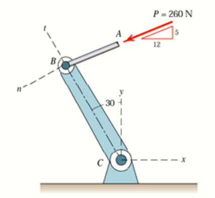
Determine the component, $F_t$ which represents a radial force at $C$ as well as the normal force $F_n$ caused by the external force vector $\mathit{\mathbf{P} }$ according to the figure.

Solution

The force is given by $\mathbf{P} = 260\dfrac{[-12, -5, 0]^T}{|[-12, -5, 0]|}$

The n-t- coordinates are given by

\begin{array}{l} t={\left\lbrack \cos \left(90\degree +30\degree \right),\sin \left(90\degree +30\degree \right),0\right\rbrack }^T \\ n={\left\lbrack \cos \left(90\degree +30\degree +90\degree \right),\sin \left(90\degree +30\degree +90\degree \right),0\right\rbrack }^T \end{array}

Then it's just a matter of projecting $\mathit{\mathbf{P} }$ onto $\mathit{\mathbf{t} }$ and $\mathit{\mathbf{n} }$

\begin{array}{l} F_t =\left(\mathit{\mathbf{P} }\cdot \mathit{\mathbf{t} }\right),\;{\mathit{\mathbf{F} } }_t =\left(\mathit{\mathbf{P} }\cdot \mathit{\mathbf{t} }\right)\mathit{\mathbf{t} }\\ F_n =\left(\mathit{\mathbf{P} }\cdot \mathit{\mathbf{n} }\right),{\;\mathit{\mathbf{F} } }_n =\left(\mathit{\mathbf{P} }\cdot \mathit{\mathbf{n} }\right)\mathit{\mathbf{n} } \end{array}

normalize = @(a)a./norm(a);
proj = @(a, b)dot(a,b)/dot(b,b)*b;
P = 260*normalize([-12, -5,0])

P = 1x3    
  -240  -100     0

t = [cosd(90+30), sind(90+30), 0]

t = 1x3    
   -0.5000    0.8660         0

n = [cosd(90+30+90), sind(90+30+90), 0]

n = 1x3    
   -0.8660   -0.5000         0

Fn = proj(P,n)

Fn = 1x3    
 -223.3013 -128.9230         0

norm(Fn)

ans = 257.8461

Ft = proj(P,t)

Ft = 1x3    
  -16.6987   28.9230         0

norm(Ft)

ans = 33.3975

Answer: $F_n \approx 258\mathrm{N},F_t \approx 33\mathrm{N}$

⚠ Note

Since

\bm n \perp \bm t

, we have that

\bm F_t + \bm F_n = \bm P

in this case.

Example 5 - Solving equations

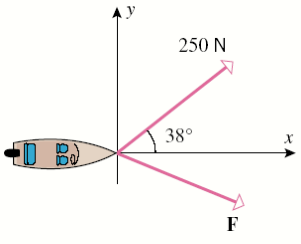
Determine the force vector $\mathit{\mathbf{F} }$ such that the resulting force on the boat is $1000.0$ N in the positive $x$ -direction.

Solution

We will make the ansatz $\mathit{\mathbf{F} }={\left\lbrack F_x \;\;F_y \;\;0\right\rbrack }^T$ and treat $F_x$ and $F_y$ as symbolic unknown variables.

The resultant:

\mathit{\mathbf{R} }=\mathit{\mathbf{F} }+250{\left\lbrack \textrm{cos38}\degree ,\textrm{sin38}\degree ,0\right\rbrack }^T ={\left\lbrack 1000.0\;\;0\;\;0\right\rbrack }^T

we get

\left\lbrack \begin{array}{c} F_x \\ F_y \\ 0 \end{array}\right\rbrack +250\left\lbrack \begin{array}{c} \textrm{cos38}\degree \\ \textrm{sin38}\degree \\ 0 \end{array}\right\rbrack =\left\lbrack \begin{array}{c} 1000.0\\ 0\\ 0 \end{array}\right\rbrack

we essentially have two unknowns and two unique equations (disregarding the 0=0 "equation"), meaning that we have a unique solution.

clear
normalize = @(a)a./norm(a);
proj = @(a, b)dot(a,b)/dot(b,b)*b;

syms F_x F_y % Declare symbolic variables
F = [F_x, F_y, 0].'

\left(\begin{array}{ccc} F_x \\ F_y \\ 0 \end{array}\right)

Resultant

R = F + 250*[cosd(38), sind(38), 0].'

\def\arraystretch{1.5} \left(\begin{array}{ccc} F_x +\frac{3465707945612477}{17592186044416} \\ F_y +\frac{2707707803577153}{17592186044416} \\ 0 \end{array}\right)

use vpa to convert to decimal and make it easier to read, five significant numbers was given, so:

R = vpa(R,5)

\left(\begin{array}{ccc} F_x +197.0 \\ F_y +153.92 \\ 0 \end{array}\right)

Now we shall solve the system of equations, we are solving for the two unknown variables $F_x$ and $F_y$ .

[F_x, F_y] = solve(R==[1000.0, 0, 0].')

\begin{align*} F_{x} & =802.99731159833027049899101257324\\ F_{y} & = -153.91536883142543956637382507324 \end{align*}

Sanitiy check:

R = vpa(subs(R),5)

\left(\begin{array}{ccc} 1000.0 \\ \text{1.875e-31} \\ 0 \end{array}\right)

vpa(norm(subs(F)),5)

817.62

Answer: $F$ needs to be 817.62N for the resulting force to be 1000.0N