Applied Mechanics

Download this page as a Matlab LiveScript

Table of contents

Introduction to Friction

We will take a look at equilibrium and friction

The box with the mass $m$ kg is exposed to an external force $P$ according to the left figure. Doing a free body diagram and applying Newton's third law reveals a force $F$ acting opposite to $P$ along the contact surface. The magnitude of this friction force depends on the type of surface and the normal force $N$. The relation between the normal force and friction force can be modelled using the Coulombs law:

$$\boxed{F\le \mu_s N}$$

where $\mu_s$ is known as the static coefficient of friction. Coulomb developed a friction theory in the 1700s for dry friction. This model assumes a linear relationship between $F$ and $N$ and even if we can empirically show that this does not generally hold for an arbitrarily large $N$, Coulombs law is taken to be "good enough" for most situations, but should be used with care.

As the force $P$ exceeds the largest possible frictional force $F_{\max }$ the box will start to slide and get an acceleration, thus the model transitions to what is known as kinetic friction and the opposing force is given by $F_k =\mu_k N$, where $\mu_k$ is the kinetic coefficient of friction. This is where statics ends and dynamics continues.

The coefficients of friction can be calculated from empirical observations using measurements of forces, positions or angles.

Here is a list for (a rough) reference

Material	$\mu_s$	$\mu_k$
Steel on steel	0.1 - 0.3	0.03 - 0.3
Steel on wood	0.5 - 0.7	0.2 - 0.5
Leather on metal	0.3 - 0.6	0.2 - 0.3
Break pad on cast iron	0.4	0.3
Hemp rope on steel	0.3	0.2
Teflon on Teflon	0.05	0.05
Rubber on metal	0.4 - 0.5	0.3 - 0.4
Rubber on asphalt	0.7 - 1.0	0.5 - 0.8
Rubber on ice	0.1	0.05

Note that Coulombs law is a very simple model in the world of tribology. Many applications need more sophisticated models of friction.

The static coefficient of friction can also be expressed as the static angle of friction, $\alpha_s$, defined by

$$\tan \left(\alpha_s \right)=\frac{F}{N}=\mu_S$$

This corresponds to the angle of a sloping plane and box that is just about to begin sliding, see Example 1.

The basic rule for analysis with friction is that the frictional force-vector $\mathit{\mathbf{F} }$ is set to be in the direction that opposes potential movement.

Essentially there two types of problem statements

1. All external forces except friction forces are known and we need to determine if the friction force can balance the external forces. This means that we need to check if $F\le \mu_s N$ in the contact surface, otherwise we have sliding and the problem is a dynamic problem with $F=\mu_k N$.

2. Some external forces are unknown and we want to know how much more we can load the body until sliding occurs. This means that we add $F_i =\mu_s N_i$ to all rough contact points and include these friction equations in the equilibrium equations. Solving for the unknown forces to answer the problem statement.

We show some typical examples involving friction.

Example 1

Determine the maximum angle $\theta$ at which the box with mass $m$ starts sliding down.

Solution:

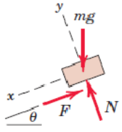
Free body diagram, where we chose the coordinate system such that most forces are aligned with the coordinate system, this minimizes expressing forces in terms of the angle.

We have equilibrium equations and an additional friction equation $F_{\max } =\mu_s N$. Then we just solve for as many variables as we have equations.

clear
syms F theta mg mu N

ekv = [mg*sin(theta) - F == 0
       -mg*cos(theta) + N == 0
       F == mu*N]

[mu,F,N] = solve(ekv, [mu,F,N])

We have $\theta =\tan^{-1} \left(\mu_s \right)$, also known as the angle of friction.

Example 2

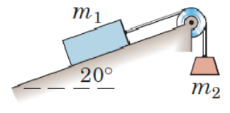
Two masses are rigged according to the figure. In what interval does $m_2$ need to be in to prevent sliding of $m_1$. Let $\mu_s =0\ldotp 3$ and $\alpha =20\degree$.

Solution:

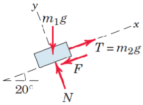
We need to examine two cases, depending on if the box is just about to start gliding up or down. These cases result in two FBDs where the direction of the friction force is opposing the direction of movement. We chose the coordinate system to be aligned to the sliding surface, since just the weight force is acting vertically. Let $F_{\max } =\mu_s N$.

Case 1: First the edge case where $m_2$ if big enough to cause sliding just to occur upwards the surface. Thus $F$ is directed against this potential movement, i.e., downwards.

clear
syms m1 m2 F g mu N alpha

FG = [-m1*g*sind(alpha); -m1*g*cosd(alpha)];
FT = [m2*g; 0];
Ff = [-F;0];
FN = [0; N];

ekv = [FG+FT+Ff+FN==0
       F==mu*N]

[F,N,m2] = solve(ekv,[F,N,m2])

alpha = 20; mu = 0.3;
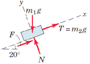
vpa(subs(m2),3)

Case 2: Then the case where $m_2$ is small enough for sliding just to occur downwards the surface. Thus $F$ is directed upwards.

syms alpha mu F N m2
Ff = [F;0];
ekv = [FG+FT+Ff+FN==0
       F==mu*N]

[F,N,m2] = solve(ekv,[F,N,m2])

alpha = 0; mu = 0.3;
vpa(subs(m2),3)

syms alpha
m2 = simplify(subs(m2)/m1)

figure
fplot(m2,[0,90]);
hold on;
fplot(0,[0,90])
xlabel('\theta'); ylabel('m_2')
title('m_2 causing sliding downwards')

vpasolve(m2==0,20)

Results

The mass $m_2$ needs to be at least $0\ldotp 06m_1$ to prevent sliding downwards and less than $0\ldotp 62m_2$ to prevent sliding upwards.

Feasibility analysis: At close to $90\degree$ the frictional force is so small that we get $m_1 =m_2$. At zero degrees the model does not work since we would get negative masses. Case 2 does not exists below slopes of ca $17\degree$, i.e., the box cannot slide downwards if the slope is less than $17\degree$.

Example 3

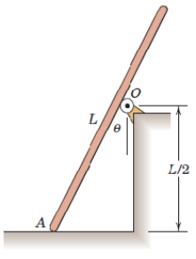
Determine the least possible $\mu_s \left(\theta \right)$ at $A$ such that the homogenous rod with a mass of $m$ does not slide. There is no friction at $O$. Disregard the radius of the roller at O. Draw a graph of $\mu_s \left(\theta \right)$ for valid angles.

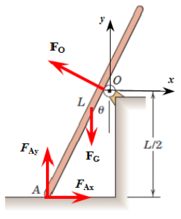
Solution: We'll start with a coordinate system according to the FBD below. Create a FBD of the rod, inserting positions vectors as needed as well as force vectors.

Define the angle using trigonometry.

$$\tan \;\theta =\dfrac{x}{L/2}=\dfrac{\sin }{\cos }$$

We start by defining the position vectors.

clear
syms L positive 
syms theta positive
% assume(theta<=90)
normalize = @(v)v/norm(v);

OA = [-L/2*sind(theta)/cosd(theta), -L/2, 0];
eAO = -normalize(OA); 
OG = OA + eAO*L/2;

The we define the force vectors acting on the rod. ${\mathit{\mathbf{F} } }_O$ is acting orthogonal to the rod. We can get its direction by using the unit circle and rotating clock-wise (adding negative angles) until we reach the desired direction. We can double check the direction by inserting values for theta. If unsure, draw the direction!

e(theta) = [cosd(theta),sind(theta),0];
syms F_O F_G F_Ax F_Ay mg
FO = F_O*e(-90-theta-90);
FA = [F_Ax, F_Ay,0];
FG = mg*[0,-1,0];

We add the equations.

ekv = [FO+FA+FG, cross(OG,FG)+cross(OA,FA)].'

[F_O, F_Ax, F_Ay] = solve(ekv,[F_O, F_Ax, F_Ay]);

simplify(F_O)

simplify(F_Ax)

simplify(F_Ay)

Since $F_{\textrm{Ax} } ={\mu F}_{\textrm{Ay} }$ we get

mu = simplify(F_Ax/F_Ay)

Note that $\theta$ must be below 90 degrees since it is limited by the length of the rod, or the A's distance to the wall. We can find the maximum value graphically, we set the length to one.

L_theta = subs(norm(OA),L,1);
figure
fplot(L_theta,[0,90]); hold on
fplot(1);
axis([0,90,0,1.1])
title('L(\theta)'); xlabel('\theta'); ylabel('L')

vpasolve(subs(norm(OA)==L,L,1),50)

You can try setting the length to any other value. Reflect on why the angle is the independent of the length.

Finally the graph on the friction coefficient as a function on the angle. $\mu_s \left(\theta \right)$ for all angles $\theta \in \left\lbrack 0,{60}^{\circ } \right\rbrack$

figure
fplot(mu,[0,60])
title('\mu_s(\theta)'); xlabel('\theta'); ylabel('\mu_s')

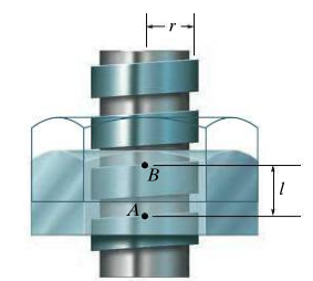
theta_max = vpasolve(diff(mu)==0,40)

mu_max = vpa(subs(mu,theta,theta_max),4)

Example 4 - Clutch

Find the relation between the applied axial force $P$ and the moment $M$ for the clutch. Assume a static case and that the friction coefficient $\mu_s =\mu$ is constant across the surface.

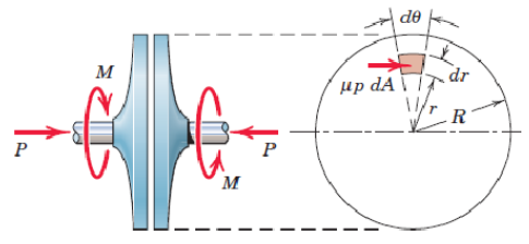
Solution: Consider the right-hand drawing where are small piece $d\theta$ of the whole ring at $r$ is drawn. The contact pressure $p$ is constant and $\textrm{dP}$ is a small contribution of $P$ i.e., the small contribution of the normal force on the ring at $r$. Now we shall take a dive into the painful details of mathematical modelling, which strengthens our skills, we define the properties of an arbitrary ring at the radius $r$.

$\textrm{dA}=2\pi \;r\;\textrm{dr}$ The area of the ring.

$\textrm{dP}=p\;\textrm{dA}$ Constant pressure.

$\textrm{dF}=\mu \;\textrm{dP}$ Fully developed friction, $\textrm{dF}\;$, acting in the tangential direction of the arrow.

$\textrm{dM}=r\;\textrm{dF}$ The contribution of the friction force to the moment, $r\bot \textrm{dF}$

clear
syms da r dr dP p dA dF mu dM dF 
[dP,dM,dF,dA]= solve([dA==2*pi*r*dr ...
                      dP==p*dA ...
                      dF==mu*dP ...
                      dM==r*dF], [dP,dM,dF,dA])

Now we can integrate, i.e., add all small bits together, where we have $P,M\;\&\;R$. Solve for the needed relations from the resulting system of equations. We'll get the surface pressure $p$ as a bonus.

$$P=\int_0^P \textrm{dP}=\int_0^R 2\pi \textrm{pr}\;\textrm{dr}$$ $$M=\int_0^M \textrm{dM}=\int_0^R 2\pi \;\mu \;p\;r^2 \;\textrm{dr}$$

syms P R M
ekv = [P == int(dP/dr, r,0,R)
       M == int(dM/dr, r,0,R)]

[M,p] = solve(ekv,[M,p])

A quick dimension analysis verifies the model and that pressure relation makes sense as well.

Example 5 - Flexible belts

Ropes and belts which are wrapped around cylinders are a very common application for static friction in mechanics. We shall look closer at the problem.

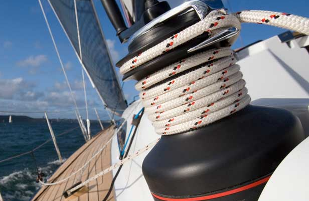
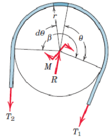
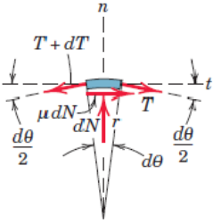
A rope is wrapped some angle $\beta \in \left\lbrack 0,\infty \right\rbrack$ radians around a cylinder. We cut a small piece $d\theta \;$ at an arbitrary angle $\theta \in \left\lbrack 0,\infty \right\rbrack$ and create a FBD according to the figure. We are interested in the maximum force and examine the limit just before sliding. The force equilibrium is divided into a tangential $\left(t\right)$ and radial $\left(n\right)$ direction

$$t:\;T\;\cos \left(\dfrac{d\theta }{2}\right)+\mu \;\textrm{dN}-\left(T+\textrm{dT}\right)\cos \left(\dfrac{d\theta }{2}\right)=0$$ $$n:\textrm{dN}-\left(T+\textrm{dT}\right)\sin \left(\dfrac{d\theta }{2}\right)-T\;\sin \left(\dfrac{d\theta }{2}\right)=0$$

Since we are dealing with very small angles, we can utilize the small angle approximation, i.e., $d\theta <<1$.

$$\overset{d\theta <<1}{\Rightarrow} \left\lbrace \begin{array}{ll} \cos \left(d\theta \right)\overset{\lim \;d\theta \to 0}{=} \;\;\;1 & \;\\ \textrm{sind}\left(d\theta \right)\overset{\lim \;d\theta \to 0}{=} \;d\theta & \; \end{array}\right.$$

Thus our expression simplifies to

$$t:\;T\;+\mu \;\textrm{dN}-\left(T+\textrm{dT}\right)=0$$ $$n:\textrm{dN}-\left(T+\textrm{dT}\right)\dfrac{d\theta }{2}-T\;\dfrac{d\theta }{2}=0$$

Since both $\textrm{dT}$ and $d\theta$ are very small, their product is even smaller and can be neglected, i.e., $\textrm{dTd}\theta <<\textrm{dT},d\theta$

Thus we end up with

$$\left\lbrace \begin{array}{ll} \mu \;\textrm{dN}=\textrm{dT} & \;\\ \textrm{dN}=T\;d\theta & \; \end{array}\right.$$

Eliminating $\textrm{dN}$ and moving thing around we can formulate a simple ordinary differential equation

$$\dfrac{ {\textrm{dT} }_2 }{d\theta }=\mu T_2$$

with the boundary condition $T_2 \left(0\right)=T_1$

For which we can easily get the solution using Matlabs symbolic differential equation solver dsolve:

clear
syms T1 T2(theta) theta mu
DE = diff(T2(theta), theta) == mu*T2(theta)

BV = T2(0)==T1

T2(theta) = dsolve(DE,BV)

$$\boxed{ T_2 = T_1 \,{\mathrm{e} }^{\mu \theta } }$$

As an alternative solution, we can collect $T$ and $\theta$ on each side: $\frac{\textrm{dT} }{T}=\mu d\theta$, and integrate:

$$\int_{T_1 }^{T_1 } \dfrac{1}{T}\textrm{dT}=\int_0^{\theta } \mu d\theta$$ $$\ln \;\dfrac{T_2 }{T_1 }=\mu \theta \Rightarrow$$ $$\boxed{ T_2 =T_1 e^{\mu \theta } }$$

Ok, so with, e.g., $\mu_s =0\ldotp 25$ (hamp against steel according to some table) and wrapped five times we get

mu = 0.25;
T2 = T1*exp(5*2*pi*mu);
vpa(T2,6)

The force $T_2$ needs to be over 2500 times larger to balance $T_1$! Now we understand why this simple mechanism works and has worked for ages!

Screws

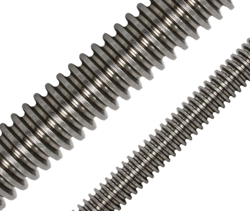
A trapezoidal screw is used for transforming a rotational movement to a linear movement. On the other hand, a common screw profile is used for maximizing axial loads. Regardless of the type of profile, the analysis is the same.

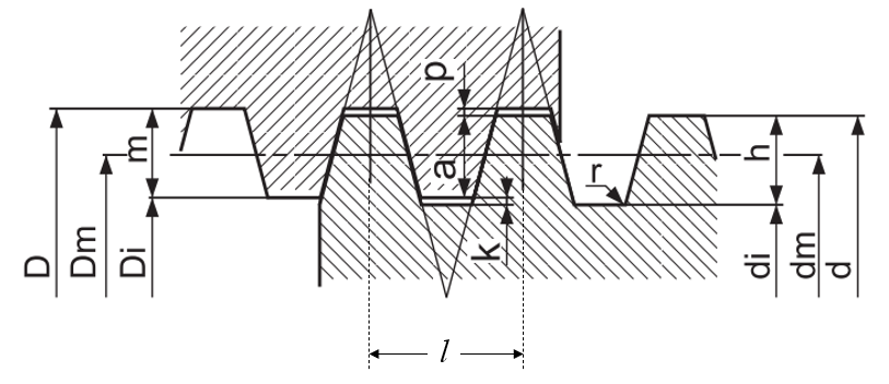
Typical measures for dimensioning are mean diameter $d_m$ and pitch $l$.

The pitch can be defined as the height increase of one rotation. Unwrapping a screw leads to the situation in the figure below.

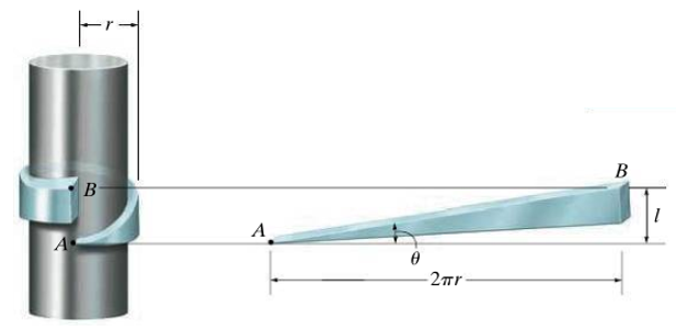
Thus, we can express the pitch-angle $\theta$ as a functin of the pitch

$$\theta =\tan^{-1} \left(\dfrac{l}{\pi d_m }\right)$$

Compared to simple bolts and screws, a trapezoidal screw has higher pitch to more efficiently transfer rotation to linear movement with fewer losses. If even more precision is needed (trapezoidal screws tend to have some backlash) then ball-screws can be used, for even less frictional losses. The tradeoff however, except the (much) higher cost of manufacturing is that ball screws can easily un-wind when an axial load is applied, thus a motor torque is needed to hold a load.

Typical pitch valued for trapezoidal screws are given tables available at various suppliers, e.g., mekanex.

Mechanical analysis

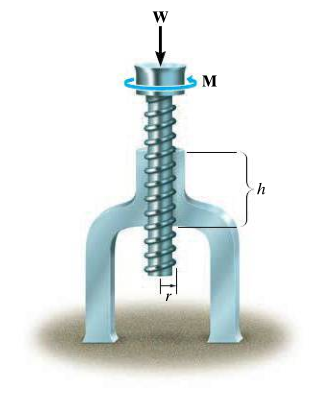
Typical questions for an analysis are: What moment $M$ is needed to transfer an axial force $W$ according to the figure above ovan given that the geometrical dimensions are $d_m ,l$ and the coefficient of friction is $\mu_s$.

We will start the analysis by looking a small cut of the screw according to the figure below.

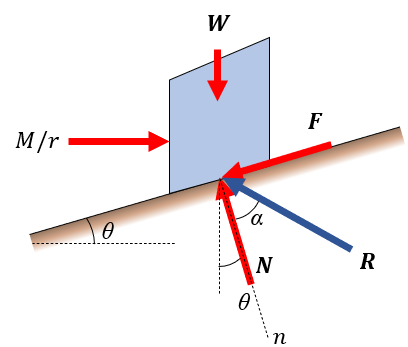
This situation describes a screw working against a load.

Sometimes the angle of friction, $\alpha$ is used, in this case the resultant, $R=F+N$ is used in the FBD.

We will not use $R$ in the following equilibrium equations.

clear
syms M r F theta N W mu

ekv = [M/r - F*cos(theta) - N*sin(theta) == 0
       N*cos(theta) - W - F*sin(theta) == 0
       F == mu*N]

[M, N, F] = solve(ekv, [M, N, F] )