Applied Mechanics

Table of contents

Constitutive relations in 2D

We shall now see how to derive the generalized Hooke's law, starting from the 1D case, we have Hooke's law.

$$\sigma_x =E\varepsilon_x$$

Now, in 2D any strain in one direction gives rise to another strain in the orthogonal direction. This is known as the transversal strain. For small strains, the transversal strain is given by

$$\varepsilon_y =-\nu \varepsilon_x$$

where $\nu$ is known as the Poisson's ratio, which is a measure of the Poisson effect and is experimentally acquired by measuring the transversal strain and the axial strain, then

$$\nu =-\dfrac{d\varepsilon_y }{d\varepsilon_x }$$

Typical values for the Poisson's ratio:

For 3D we get

$$\def\arraystretch{2.0} \left.\begin{array}{c} \varepsilon_x =\dfrac{\sigma_x }{E}-\nu \left(\dfrac{\sigma_y }{E}+\dfrac{\sigma_z }{E}\right)\\ \varepsilon_y =\dfrac{\sigma_y }{E}-\nu \left(\dfrac{\sigma_x }{E}+\dfrac{\sigma_z }{E}\right)\\ \varepsilon_z =\dfrac{\sigma_z }{E}-\nu \left(\dfrac{\sigma_x }{E}+\dfrac{\sigma_y }{E}\right) \end{array}\right\rbrace \left\lbrack \begin{array}{c} \varepsilon_x \\ \varepsilon_y \\ \varepsilon_z \end{array}\right\rbrack =\dfrac{1}{E}\left\lbrack \begin{array}{ccc} 1 & -\nu & -\nu \\ -\nu & 1 & -\nu \\ -\nu & -\nu & 1 \end{array}\right\rbrack \left\lbrack \begin{array}{c} \sigma_x \\ \sigma_y \\ \sigma_z \end{array}\right\rbrack$$

This system can be inverted, yielding

$$\def\arraystretch{2.0} \begin{array}{l} \sigma_x =\dfrac{E}{1+\nu }\left(\varepsilon_x +\dfrac{\nu }{1+2\nu }\left(\varepsilon_x +\varepsilon_y +\varepsilon_z \right)\right)\\ \sigma_y =\dfrac{E}{1+\nu }\left(\varepsilon_y +\dfrac{\nu }{1+2\nu }\left(\varepsilon_x +\varepsilon_y +\varepsilon_z \right)\right)\\ \sigma_z =\dfrac{E}{1+\nu }\left(\varepsilon_z +\dfrac{\nu }{1+2\nu }\left(\varepsilon_x +\varepsilon_y +\varepsilon_z \right)\right) \end{array}$$

Bulk modulus

The bulk modulus, $K$ is defined as pressure over volume change and is a measure of how resistant to compression a material is.

$$K=\dfrac{\sigma_m }{\Delta }$$

using $\Delta =\varepsilon_x +\varepsilon_y +\varepsilon_z$, i.e., total volume strain

we get

$$\Delta =\dfrac{1-2\nu }{E}\left(\sigma_x +\sigma_y +\sigma_z \right)$$

under the same pressure we have

$$\sigma_x +\sigma_y +\sigma_z =3\sigma_m$$

and thus

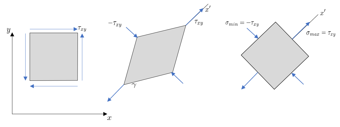
$$K=\dfrac{\sigma_m }{\Delta }=\dfrac{E}{3\left(1-2\nu \right)}$$

Shear modulus

Consider an element under pure shear. We can rotate this element such that the shear stresses align with the principal stresses.

$\sigma_{\max } =\sigma_1 =\tau_{x\;y}$, $\sigma_{\min } =\sigma_2 =-\tau_{x\;y}$

We can substitute the normal stresses with principal stresses, $\sigma_x =\sigma_{\max } ,\sigma_y =\sigma_{\min } ,\sigma_z =0$ into the equation

$$\begin{array}{l} \varepsilon_x =\dfrac{\sigma_x }{E}-\nu \left(\dfrac{\sigma_y }{E}+\dfrac{\sigma_z }{E}\right)=\varepsilon_{\max } =\dfrac{\tau_{x\;y} }{E}-\nu \left(\dfrac{-\tau }{E}+0\right)\\ \Rightarrow \varepsilon_{\max } =\dfrac{\tau_{x\;y} }{E}\left(1+\nu \right) \end{array}$$

Similar to the principal stresses, we can get the principal strains

$$\varepsilon_{1,2} =\dfrac{\varepsilon_x +\varepsilon_y }{2}\pm \sqrt{ {\left(\dfrac{\varepsilon_x +\varepsilon_y }{2}\right)}^2 +{\left(\dfrac{\gamma_{x\;y} }{2}\right)}^2 }$$

and in the principal direction we have $\varepsilon_x =\varepsilon_y =0$

and thus the strain in the principal direction is

$$\varepsilon_{\max } =\varepsilon_1 =\dfrac{\gamma_{x\;y} }{2}$$

Hooke's law for shearing states that

$$\tau_{x\;y} =G\gamma_{x\;y}$$

So we get $\varepsilon_{\max } =\frac{\tau_{x\;y} }{2G}$, and thus

$$G=\dfrac{E}{2\left(1+\nu \right)}$$

Generalized Hooke's law

In general we have $\varepsilon =\frac{\tau_{x\;y} }{2G}$ which leads to

$$\varepsilon_{x\;y} =\left(1+\nu \right)\dfrac{\tau_{x\;y} }{E}$$

and

$$\tau_{x\;y} =\dfrac{E}{1+\nu }\varepsilon_{x\;y}$$

Since earlier we have

$$\sigma_x =\dfrac{E}{1+\nu }\left(\varepsilon_x +\dfrac{\nu }{1+2\nu }\left(\varepsilon_x +\varepsilon_y +\varepsilon_z \right)\right)$$

which when expanded becomes

$$\sigma_x =\left(\underset{2\mu =2G}{\underbrace{\dfrac{E}{1+\nu } } } \varepsilon_x +\underset{\lambda }{\underbrace{\dfrac{E\nu }{\left(1+\nu \right)\left(1+2\nu \right)} } } \left(\varepsilon_x +\varepsilon_y +\varepsilon_z \right)\right)$$

we recognize, in the first term, the shear modulus $G$, also denoted $\mu$. In the second term we identify the parameter $\lambda$. The parameters $\lambda$ and $\mu$ are known as the Lamé parameters. Using these parameters we can simplify the stress and generalize it into a matrix

$$\left\lbrack \begin{array}{ccc} \sigma_x & \tau_{x\;y} & \tau_{x\;z} \\ \tau_{x\;y} & \sigma_y & \tau_{y\;z} \\ \tau_{x\;z} & \tau_{y\;z} & \sigma_z \end{array}\right\rbrack =2\mu \left\lbrack \begin{array}{ccc} \varepsilon_x & \varepsilon_{x\;y} & \varepsilon_{x\;z} \\ \varepsilon_{x\;y} & \varepsilon_y & \varepsilon_{y\;z} \\ \varepsilon_{x\;z} & \varepsilon_{y\;z} & \varepsilon_z \end{array}\right\rbrack +\lambda \underset{\mathit{\mathbf{I} } }{\underbrace{\left\lbrack \begin{array}{ccc} 1 & 0 & 0\\ 0 & 1 & 0\\ 0 & 0 & 1 \end{array}\right\rbrack } } \underset{\mathrm{tr}\varepsilon =\nabla \cdot \mathit{\mathbf{u} } }{\underbrace{\left(\varepsilon_x +\varepsilon_y +\varepsilon_z \right)} }$$

A quick sanity check: $\sigma_y =2\mu \varepsilon_y +\lambda \left(\varepsilon_x +\varepsilon_y +\varepsilon_z \right)$ and $\tau_{x\;z} =2\mu \varepsilon_{x\;z}$.

We arrive at the generalized Hooke´s law for isotropic materials

$$\sigma =2\mu \varepsilon +\lambda \mathrm{tr}\varepsilon \mathit{\mathbf{I} }\;\mathrm{or}\;\sigma =2\mu \varepsilon +\lambda \nabla \cdot \mathit{\mathbf{u} }\;\mathit{\mathbf{I} }$$

Note that the notation for the shear modulus $G$ has an solid mechanics background whereas $\mu$ comes from continuum mechanics.

The first term of the stress tensor is known as the deviatoric stress tensor and the second term is known as the volumetric stress tensor. The same goes for the strain tensor.

$$\varepsilon =\dfrac{1}{2\mu }\sigma -\dfrac{\lambda }{2\mu \left(3\lambda +2\mu \right)}\mathrm{tr}\sigma \mathit{\mathbf{I} }$$

The Efficient Engineer video on this topic.

Volumetric strain and incompressibility

Consider a cube with side length $a$, the total change in volume (under small strain assumption) is

$$\Delta V=V-V_0 \approx a^3 \left(1+\varepsilon_x +\varepsilon_y +\varepsilon_z \right)$$

where we identify the dilation of the volume as $\varepsilon_x +\varepsilon_y +\varepsilon_z =\mathrm{tr}\varepsilon =:I_1$, also known as the first invariant of the strain tensor.

Now, consider $\lambda$ in the generalized Hooke's law, $\lambda =\frac{E\nu }{\left(1+\nu \right)\left(1+2\nu \right)}$, and note that as $\nu \to 1/2$ we get

$\lambda \to \infty \overset{\mathrm{forcing} }{\Rightarrow} \varepsilon_x +\varepsilon_y +\varepsilon_z \to 0$.

Which means that the volume change tends to zero with the Poisson's ratio tending towards 0.5, meaning the material becomes incompressible.

2D Simplifications

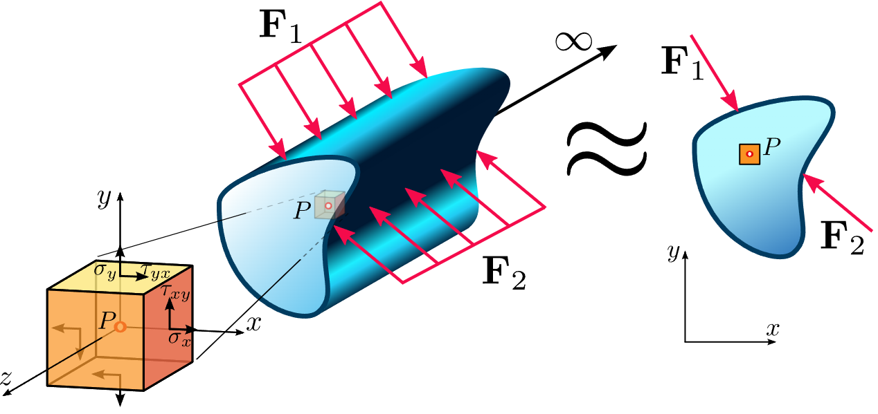
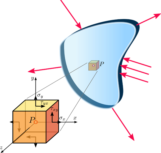
Many applications where the structure is much longer than its cross section can be approximated using a 2D simplification called plain strain. This greatly reduces the computational complexity of solving the resulting numerical problem.

Plain strain

For plain strain all strain components in the $z-$direction vanish due to the much longer $z-$dimension and thus the strain tensor simplifies to

$$\left\lbrack \begin{array}{ccc} \varepsilon_x & \varepsilon_{x\;y} & 0\\ \varepsilon_{x\;y} & \varepsilon_x & 0\\ 0 & 0 & 0 \end{array}\right\rbrack$$

which gives

$$\left\lbrack \begin{array}{ccc} \sigma_x & \sigma_{x\;y} & 0\\ \sigma_{x\;y} & \sigma_x & 0\\ 0 & 0 & \sigma_z \end{array}\right\rbrack$$

The stress tensor has a non-zero z component due to: $\sigma_z =\frac{E}{1+\nu }\left(0+\frac{\nu }{1+2\nu }\left(\underset{\not= 0}{\underbrace{\varepsilon_x +\varepsilon_y } } +0\right)\right)$.

Hooke's law takes the form

$$\left\lbrack \begin{array}{cc} \sigma_x & \sigma_{x\;y} \\ \sigma_{x\;y} & \sigma_y \end{array}\right\rbrack =\dfrac{E}{1+\nu }\left(\left\lbrack \begin{array}{cc} \varepsilon_x & \varepsilon_{x\;y} \\ \varepsilon_{x\;y} & \varepsilon_y \end{array}\right\rbrack +\dfrac{\nu }{1+2\nu }\left\lbrack \begin{array}{cc} 1 & 0\\ 0 & 1 \end{array}\right\rbrack \left(\varepsilon_x +\varepsilon_y \right)\right)$$

with the Lamé parameters

$$\lambda =\dfrac{E\nu }{\left(1+\nu \right)\left(1+2\nu \right)}\;\mathrm{and}\;\mu =\dfrac{E}{2\left(1+\nu \right)}$$

Plane stress

For plane stress, we assume a very thin object that is loaded in-plane. No bending can occur in such a model. Typical applications are thin walled structures with edge loads, even very slightly curved geometry can assume plane stress, such as pressure vessels. This type of model is also called a plate. The stress can be simplified to

$$\left\lbrack \begin{array}{ccc} \sigma_x & \sigma_{x\;y} & 0\\ \sigma_{x\;y} & \sigma_x & 0\\ 0 & 0 & 0 \end{array}\right\rbrack$$

effectively reducing the problem to a 2D problem.

Hooke's law takes the form

$$\left\lbrack \begin{array}{cc} \sigma_x & \sigma_{x\;y} \\ \sigma_{x\;y} & \sigma_y \end{array}\right\rbrack =\dfrac{E}{1-\nu^2 }\left(\left(1-\nu \right)\left\lbrack \begin{array}{cc} \varepsilon_x & \varepsilon_{x\;y} \\ \varepsilon_{x\;y} & \varepsilon_y \end{array}\right\rbrack +\nu \left\lbrack \begin{array}{cc} 1 & 0\\ 0 & 1 \end{array}\right\rbrack \left(\varepsilon_x +\varepsilon_y \right)\right)$$

In this case, the Lamé parameter become

$$\lambda =\dfrac{E\nu }{1+\nu^2 }\;\mathrm{and}\;\mu =\dfrac{E}{2\left(1+\nu \right)}$$

Note however that we have a non-zero strain component due to

$$\varepsilon_z =0-\nu \left(\dfrac{\sigma_x }{E}+\dfrac{\sigma_y }{E}\right)$$

Videos on the topic

Make sure to check out The Efficient Engineers video on this topic