GoldenQuad

Table of contents

The Golden Quad
Example 1
Example 2

The Golden Quad

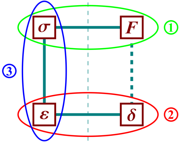
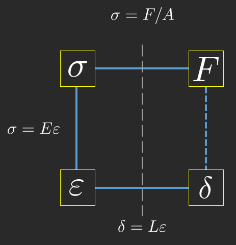
On the right side we have external quantities, such as the load $F$ and deformation $\delta$ (or displacement $u$ ). On the left side we have internal quantities, such as the stress $\sigma$ and strain $\varepsilon$ .

The golden quad provides the three relations:

Equilibrium, which connects loads to stresses. These relations are formulated by mechanics and creating a free body diagram and posing the equilibrium equations.

Deformation relations, these connect deformations to strains and are purely geometric. These are sometimes called kinematic relations. Typically something is known on the boundary, which is introduced as a kinematic relation.

Material relations, or constitutive relations, these connect the strains to the stresses using knowledge about the material which is acquired experimentally. Typically material parameters are Young's modulus $E$ , Poisson's ratio $\nu$ and the thermal expansion coefficient $\alpha$ .

The workflow using the golden quad is:

Formulate all relations, 1,2,3, according to the figure. This is mechanics, solid mechanics, modeling and computational thinking.
Solve the resulting system of equations. This is not mechanics or solid mechanics, but rudimentary mathematics which is best left to the computer to solve using your favorite technical programming language.

\left\lbrace \begin{array}{ll} \sigma =F/A & \\ \sigma =E\varepsilon & \\ \delta =L\varepsilon & \end{array}\right.\Rightarrow \delta =\dfrac{F\;L}{E\;A}

Bodies in series:

\delta =\sum \delta_i =\sum \dfrac{N_i L_i }{E_i A_i }

Example 1

A linear elastic rod is fastened between two rigid walls and exposed to heating. Determine the stress and reaction forces on the walls.

Solution

Cut and free body diagram

\left\lbrace \begin{array}{ll} N-P=0,\sigma =N/A & \textrm{Equilibrium}\;\textrm{equations}\\ \varepsilon_{\textrm{tot} } =\delta /L,\delta =0 & \textrm{Deformation},\delta =0\;\textrm{boundary}\;\textrm{condition}\\ \sigma =E\varepsilon_{\textrm{elast} } & \textrm{Material},\textrm{elastic}\;\textrm{relation}\\ \varepsilon_T =\alpha \Delta T & \textrm{Thermal}\;\textrm{strain}\\ \varepsilon_{\textrm{tot} } ={\varepsilon_{\textrm{elast} } +\varepsilon }_T & \textrm{Total}\;\textrm{strain} \end{array}\right.

From this system of equations we get 7 unknowns of which these are the ones we are interested in:

$P=-E\;A\;\alpha \Delta T$ , $\sigma =-E\;\alpha \Delta T$

dimension analysis checks out and we clearly see that we have negative force and stress as it should be.

Example 2

Same problem as above but two different rods and materials.

Solution:

\left\lbrace \begin{array}{ll} -S_1 +N_1 =0,-N_1 +N_2 =0,-N_2 +S_2 =0 & \textrm{Equilibrium}\;\textrm{equations}\\ \sigma_1 =N_1 /A_1 ,\sigma_2 =N_2 /A_2 & \textrm{Equilibrium}\;\textrm{equations}\\ \varepsilon_{E1} =\delta_1 /L_1 ,\varepsilon_{E2} =\delta_2 /L_2 ,\delta_1 +\delta_2 =0 & \textrm{Deformation}\;\textrm{and}\;\textrm{boundary}\;\textrm{condition}\\ \sigma_1 =E\varepsilon_{E1} ,\sigma_2 =E\varepsilon_{E2} & \textrm{Material},\textrm{elastic}\;\textrm{relation}\\ \varepsilon_{\textrm{T1} } =\alpha_1 \Delta T,\varepsilon_{\textrm{T2} } =\alpha_2 \Delta T & \textrm{Thermal}\;\textrm{strain}\\ \varepsilon_{\textrm{tot1} } =\varepsilon_{\textrm{E1} } +\varepsilon_{\textrm{T1} } ,\varepsilon_{\textrm{tot2} } =\varepsilon_{\textrm{E2} } +\varepsilon_{\textrm{T2} } & \textrm{Total}\;\textrm{strain} \end{array}\right.

We now have 14 equations and 14 unknowns from which we can determine the stress in the two bodies and the reaction forces.

© Mirza Cenanovic. Last modified: April 17, 2024. Website built with Franklin.jl and the Julia programming language.