Shaft3D

Table of contents

Description
Modeling - Kinematics
Verification
Visualization
Symbolic model
Rotating around a local axis

Description

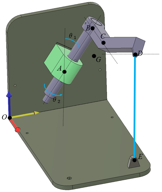
Working in 3D is not too difficult once we get familiar with proper tools. Here we shall give a thorough walk-through of the process on a non-trivial example. The hardest part is the kinematics, i.e., describing the positions of the points relative to each other. Once this is done, formulating forces and moments to do equilibrium is a trivial matter with computer support.

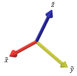
We shall here learn to work with a rotated coordinate system.

$\textrm{OA}={\left\lbrack 30,60,75\right\rbrack }^T \textrm{mm}$ , $L_{\textrm{AB}} =65$ , $L_{\textrm{BC}} =50\textrm{mm}$ , $\theta_1 =35\;^\circ$ around the local $x$ -axis at $A$ and $E=\left(145,40,0\right)$

Let $\theta_2$ denote the rotation of the shaft $\textrm{AB}$ . In the picture above, the $\overrightarrow{\textrm{BC}}$ vector is parallel to the $x-$ axis, and this is when $\theta_2 =0^{\circ }$ .

The center of gravity can be defined using local coordinates as: $\overrightarrow{\textrm{AG}} =34\tilde{x} +51\tilde{z}$

Similarly, we can define $\overrightarrow{CD}=70\tilde{\bm x} +40\tilde{\bm z}$ using local coordinates. See below for the definition of the local coordinates.

Given the spring constant of $k=0.1$ N/mm and the unloaded spring length of $L_0 =120$ mm:

Determine and plot the length of the spring $L_{DE}(\theta_2)$ as well as the spring force $F(\theta_2)$ .
Determine and plot the moment which the motor needs to generate to rotate the shaft AB, $M_{AB}(\theta_2)$ for $\theta_2 \in [ 90^\circ,-90^\circ ]$

Modeling - Kinematics

We are going to work with vectors to define the path from $O$ to $D$ and $G$ as a function of the rotation angle $\theta$ . To do this with our sanity in tact, we will introduce local coordinates and rotate these using rotation matrices.

R_x \left(\theta \right)=\left\lbrack \begin{array}{ccc} 1 & 0 & 0\\ 0 & \cos \theta & -\sin \theta \\ 0 & \sin \theta & \cos \theta \end{array}\right\rbrack

R_y \left(\theta \right)=\left\lbrack \begin{array}{ccc} \cos \theta & 0 & \sin \theta \\ 0 & 1 & 0\\ -\sin \theta & 0 & \cos \theta \end{array}\right\rbrack

R_z \left(\theta \right)=\left\lbrack \begin{array}{ccc} \cos \theta & -\sin \theta & 0\\ \sin \theta & \cos \theta & 0\\ 0 & 0 & 1 \end{array}\right\rbrack

We shall introduce the local vectors $\tilde{\bm x} ,\tilde{\bm y}$ and $\tilde{\bm z}$ and always let $\tilde{\bm z}$ point in the direction of the path.

We start by getting to point $A$ using the vector $\overrightarrow{OA}$ . From here we need to establish the direction of the shaft axis, which we can do by rotating the $\bm z$ vector around the $x$ -axis by ${-\theta }_1$ degrees (using the right hand rule).

This gives our $\bm e_{AB}$ direction.

\bm e_{AB} =\tilde{\bm z} ={\bm R}_x \left(\theta_1 \right)\;{\bm e}_z

clear
ez = [0;0;1];
R_x = @(a) [1 0         0
            0 cosd(a)  -sind(a)
            0 sind(a)   cosd(a)];

R_y = @(a) [cosd(a)  0  sind(a)
            0        1  0
            -sind(a) 0  cosd(a)];

R_z = @(a) [cosd(a)  -sind(a)  0
            sind(a)   cosd(a)  0
            0         0        1];

theta1 = 35; theta2 = 30;
eAB = R_x(-theta1)*ez

⚠ Note

Note that we rotate

-\theta_1

due to the right hand rule, i.e., put the thumb in the direction of

x

and the fingers will point in the positive direction of rotation.

The shaft $\textrm{AB}$ needs to rotate around its axis, or the $\tilde{z} -\textrm{axis}$ . The rotation can be achieved by rotating around the global axis, $x,y\;$ and $z$ . From the initial configuration, see below, where the shaft axis is aligned with the $z$ -axis and $\overrightarrow{BC}$ oriented towards the $x$ -axis. To get the correct rotation of the shaft, we need to first rotate around the $z$ -axis and then around the $x$ -axis.

1: First we rotate around the

z

axis.

2: Then we rotate around the

x

axis.

Mathematically, this is the same as rotating our coordinate system by

\tilde{\bm X} =\left\lbrack \tilde{\bm x} ,\tilde{\bm y} ,\tilde{\bm z} \right\rbrack ={\bm R}_x \left(-\theta_1 \right){\bm R}_z \left(\theta_2 \right)\bm I

where $\bm I$ is the identity matrix containing the Cartesian bases, i.e.,

\left\lbrack {\bm e}_x ,{\bm e}_y ,{\bm e}_z \right\rbrack =\left\lbrack \begin{array}{ccc} 1 & 0 & 0\\ 0 & 1 & 0\\ 0 & 0 & 1 \end{array}\right\rbrack

Verification

Let us verify this by setting $\theta_1 =0\;$ and $\theta_2 =0$ , we expect $\tilde{\bm X} =\bm I$

theta1 = 0; theta2 = 0;
X = R_x(theta1)*R_z(theta2)*eye(3)

X = 3x3    
     1     0     0
     0     1     0
     0     0     1

Now we can set $\theta_2 =90$ and we should have that $\tilde{\bm x} ={\left\lbrack 0\;1\;0\right\rbrack }^T$

theta1 = 0; theta2 = 90;
X = R_x(theta1)*R_z(theta2)*eye(3)

X = 3x3    
     0    -1     0
     1     0     0
     0     0     1

We can confirm this and also see that $\tilde{\bm y} ={\left\lbrack -1\;0\;0\right\rbrack }^T$ as it should.

Now we can rotate around the $x-\textrm{axis}$ by $\theta_1 =-90$ , we should get $\tilde{z} ={\left\lbrack 0\;1\;0\right\rbrack }^T$

theta1 = -90; theta2 = 90;
X = R_x(theta1)*R_z(theta2)*eye(3)

X = 3x3    
     0    -1     0
     0     0     1
    -1     0     0

We can confirm that the new coordinates point in the expected directions.

Thus have confirmed that the rotation makes sense, we have built confidence in our model and can set the rotation to solve our problem:

theta1 = -35; theta2 = 0;
X = R_x(theta1)*R_z(theta2)*eye(3)

X = 3x3    
    1.0000         0         0
         0    0.8192    0.5736
         0   -0.5736    0.8192

eex = X(:,1); eey = X(:,2); eez = X(:,3);

Now we can easily model the rest of the points.

\begin{array}{l} \overrightarrow{\textrm{AB} } =L_{\textrm{AB} } \tilde{\bm z} \\ \overrightarrow{\textrm{BC} } =L_{\textrm{BC} } \tilde{\bm x} \\ \overrightarrow{\textrm{CD} } =70\tilde{\bm x} +40\tilde{\bm z} \\ \overrightarrow{\textrm{AG} } =34\tilde{\bm x} +51\tilde{\bm z} \\ \overrightarrow{\textrm{DE} } = \overrightarrow{\textrm{OE} }- \overrightarrow{\textrm{OD} } \end{array}

Visualization

We do a final verification of the kinematics by visualizing the geometry in Matlab:

OA = [30, 60, 75]';    % mm
OE = [175, 105, 15]';  % mm
L_AB = 65;             % mm
L_BC = 50;             % mm
k = 0.2;               % N/mm
L0 = 120;              % mm
theta1 = 35;           % deg
theta2 = 26;           % deg

X = R_x(-theta1)*R_z(theta2)*eye(3);
eex = X(:,1); eey = X(:,2); eez = X(:,3);

AB = eez*L_AB;
BC = eex*L_BC;
CD = eex*70 + eez*40;

OD = OA + AB + BC + CD;
OB = OA+AB;
OC = OB+BC;
AD = OD - OA;
DE = OE - OD;

AG = 34*eex + 51*eez;
OG = OA + AG;

% Visualization
close all
figure
axis equal; hold on;
xlabel('x'); ylabel('y'); zlabel('z');
set(gcf,'Visible','on')

hp1 = plot3([OA(1), OB(1)], ...
            [OA(2), OB(2)], ...
            [OA(3), OB(3)], '-k', 'LineWidth',2);
htA = text(OA(1), OA(2), OA(3), 'A');
htB = text(OB(1), OB(2), OB(3), 'B');

hp2 = plot3([OB(1), OC(1)], ...
            [OB(2), OC(2)], ...
            [OB(3), OC(3)], '-k', 'LineWidth',2);
htC = text(OC(1), OC(2), OC(3), 'C');

hp3 = plot3([OC(1), OD(1)], ...
            [OC(2), OD(2)], ...
            [OC(3), OD(3)], '-k', 'LineWidth',2);
htD = text(OD(1), OD(2), OD(3), 'D');

hp4 = plot3([OD(1), OE(1)], ...
            [OD(2), OE(2)], ...
            [OD(3), OE(3)], '-m', 'LineWidth',2);
htE = text(OE(1), OE(2), OE(3), 'E');

hp5 = plot3(OG(1), OG(2), OG(3), 'ok', 'MarkerFaceColor','k');

view(3)

grid on
axis([0,200, -100, 250, 0, 250])
view(-69, 35)
view(2)
view(40, 32)
htitel = title(sprintf('$\\theta=%d^\\circ$',theta2),'interpreter','latex');

% Animation below

% exportgraphics(gca,"shaft3D.gif","Append",false)
% 
% Az = [52, 80];
% El = [44, 74];
% 
% view(52,44)
% Theta = [-90:1:90, 89:-1:-90];
% c = 1;
% 
% for theta2 = Theta
%     t = c/length(Theta);
%     az = Az(1) + t*(Az(2)-Az(1));
%     el = El(1) + t*(El(2)-El(1));
%     view(az,el)
% 
%     X = R_x(-theta1)*R_z(theta2)*eye(3);
%     eex = X(:,1); eey = X(:,2); eez = X(:,3);
% 
%     AB = eez*L_AB;
%     BC = eex*L_BC;
%     CD = eex*70 + eez*40;
% 
%     OD = OA + AB + BC + CD;
%     OB = OA+AB;
%     OC = OB+BC;
%     AD = OD - OA;
%     DE = OE - OD;
% 
%     AG = 34*eex + 51*eez;
%     OG = OA + AG;
% 
%     set(hp1, 'XData', [OA(1), OB(1)], ...
%              'YData', [OA(2), OB(2)], ...
%              'ZData', [OA(3), OB(3)]);
%     set(hp2, 'XData', [OB(1), OC(1)], ...
%              'YData', [OB(2), OC(2)], ...
%              'ZData', [OB(3), OC(3)])
%     set(hp3, 'XData', [OC(1), OD(1)], ...
%              'YData', [OC(2), OD(2)], ...
%              'ZData', [OC(3), OD(3)])
%     set(hp4, 'XData', [OD(1), OE(1)], ...
%              'YData', [OD(2), OE(2)], ...
%              'ZData', [OD(3), OE(3)])
%     set(hp5, 'XData', OG(1), 'YData', OG(2), 'ZData', OG(3))
%     set(htA, 'Position', [OA(1),OA(2), OA(3)])
%     set(htB, 'Position', [OB(1),OB(2), OB(3)])
%     set(htC, 'Position', [OC(1),OC(2), OC(3)])
%     set(htD, 'Position', [OD(1),OD(2), OD(3)])
%     set(htE, 'Position', [OE(1),OE(2), OE(3)])
%     set(htitel,'String', sprintf('$\\theta=%d^\\circ$',theta2))
%     drawnow
%     c = c+1;
%     exportgraphics(gca,"shaft3D.gif","Append",true)
% end

The spring force is modeled using

L=|\overrightarrow{\textrm{DE} } |,{\bm e}_{\textrm{DE} } =\dfrac{\overrightarrow{\textrm{DE} } }{L},L_0 =120\textrm{mm}

F=k\left(L-L_0 \right)\;\textrm{and}\;\bm F=F\;{\bm e}_{\textrm{DE} }

The moment at $A$ is the given by

{\bm M}_A =\overrightarrow{\textrm{AD} } \times \bm F+\overrightarrow{\textrm{AG} } \times \bm W

where $\bm W={\left\lbrack 0,0,-m\;g\right\rbrack }^T$ where $m=150\;$ g, and

\overrightarrow{\textrm{AD} } =\overrightarrow{\textrm{OD} } -\overrightarrow{\textrm{OA} }

Finally the moment around the axis is given by

M_{\textrm{AB} } ={\bm M}_A \cdot \tilde{\bm z}

Symbolic model

Now we can plot the graphs using a symbolic $\theta_2$

syms theta2 real

X = R_x(-theta1)*R_z(theta2)*eye(3);
eex = X(:,1); eey = X(:,2); eez = X(:,3);

AB = eez*L_AB;
BC = eex*L_BC;
CD = eex*70 + eez*40;

OD = OA + AB + BC + CD;
OB = OA+AB;
OC = OB+BC;
AD = OD - OA;
DE = OE - OD;

AG = 34*eex + 51*eez;
OG = OA + AG;

L = norm(DE);
eDE = DE/L;

L0 = 120;
F = k*(L-L0);
FF = F*eDE;

W = [0; 0; -0.15*9.82];

figure
fplot(L,[-90,90])
xlabel('\theta [deg]')
ylabel('L [mm]')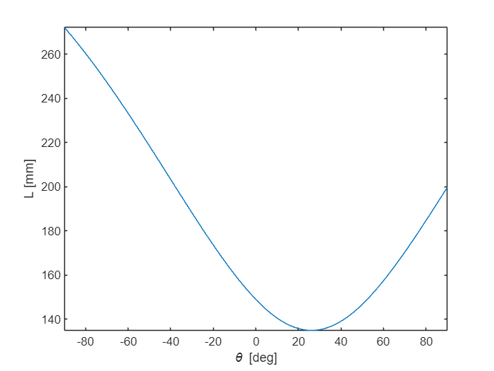

figure
fplot(F,[-90,90])
xlabel('\theta [deg]')
ylabel('F [N]')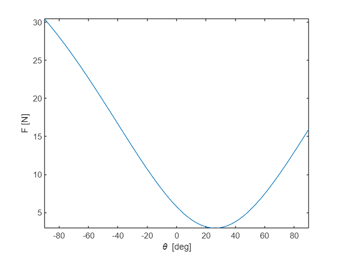

M_A = cross(AD, FF) + cross(AG, W);

eAB = eez;

M_AB = dot(M_A, eAB)/1000;
figure
fplot(M_AB,[-90,90])
xlabel('\theta [deg]')
ylabel('M [Nm]')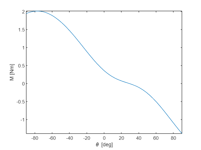

Zooming in at the force graph, we learn that the minimum force and length of the spring occurs at $26^\circ$ .

The maximum moment occurs at around $-78^\circ$ . The moment is zero around $29.5^\circ$ .

Rotating around a local axis

Another approach to rotating the coordinate system is to rotate around a local coordinate system. This makes the modeling and thinking easier. One does not need to be confined to thinking about rotations around global coordinates.

This can be done by rotating the $z$ -rotation matrix, $\bm R_z$ around the $x$ -axis by:

\bm R_{\tilde z}(\theta_2) = \bm R_x(\theta_1) \bm R_z(\theta_2)

This rotation matrix rotates vectors around the $\tilde z$ axis. This approach still relies on defining the rotation matrix by rotating it around global axis. The order of rotations is important, thus chaining rotations can become tedious.

It would be nicer to have a function that lets us rotate around a arbitrary vector $\bm u$ . To achieve this we visit our favorite source of goodyness, Wikipedia, and find that the very elegant way of rotating a vector $\bm v$ around an axis $\bm u$ by an angle $\theta$ according to the right-hand rule is stated as

{\bm R}_u \bm v=\bm u\;\left(\bm u\cdot \bm v\right)+\cos \theta \left(\bm u\times \bm v\right)\times u+\sin \theta \left(\bm u\times \bm v\right)

which we can write in matlab as

Ruv = @(a,u,v) u*dot(u,v) + cross(cosd(a)*cross(u,v), u) + sind(a)*cross(u,v);

We can test this by rotating the $x$ -axis 90 degrees around and $z$ -axis, we expect the resulting vector to be ${\left\lbrack 0,1,0\right\rbrack }^T$

Ruv(90,[0;0;1],[1;0;0])

Now we can repeat the definitions of the points from the example above using the new rotation tool.

OA = [30, 60, 75]';    % mm
OE = [175, 105, 15]';  % mm
L_AB = 65;             % mm
L_BC = 50;             % mm
k = 0.2;               % N/mm
L0 = 120;              % mm
theta1 = 35;           % deg
theta2 = 26;           % deg

We formulate the direction $\bm e_{AB}$ by rotating the $z$ -axis around the $x$ -axis.

eAB = Ruv(-theta1, [1,0,0]', [0,0,1]')
eez = eAB;

Ok, nothing new, hardly easier than using standard rotation matrices. But now we can rotate around $\bm e_{AB}$

eex = Ruv(theta2, eAB, [1,0,0]')

AB = eez*L_AB;
BC = eex*L_BC;
CD = eex*70 + eez*40;

OD = OA + AB + BC + CD;
OB = OA+AB;
OC = OB+BC;
AD = OD - OA;
DE = OE - OD;

AG = 34*eex + 51*eez;
OG = OA + AG;

% Visualization
close all
figure
axis equal; hold on;
xlabel('x'); ylabel('y'); zlabel('z');
set(gcf,'Visible','on')

hp1 = plot3([OA(1), OB(1)], ...
            [OA(2), OB(2)], ...
            [OA(3), OB(3)], '-k', 'LineWidth',2);
htA = text(OA(1), OA(2), OA(3), 'A');
htB = text(OB(1), OB(2), OB(3), 'B');

hp2 = plot3([OB(1), OC(1)], ...
            [OB(2), OC(2)], ...
            [OB(3), OC(3)], '-k', 'LineWidth',2);
htC = text(OC(1), OC(2), OC(3), 'C');

hp3 = plot3([OC(1), OD(1)], ...
            [OC(2), OD(2)], ...
            [OC(3), OD(3)], '-k', 'LineWidth',2);
htD = text(OD(1), OD(2), OD(3), 'D');

hp4 = plot3([OD(1), OE(1)], ...
            [OD(2), OE(2)], ...
            [OD(3), OE(3)], '-m', 'LineWidth',2);
htE = text(OE(1), OE(2), OE(3), 'E');

hp5 = plot3(OG(1), OG(2), OG(3), 'ok', 'MarkerFaceColor','k');

view(3)

grid on
axis([0,200, -100, 250, 0, 250])
view(-69, 35)
view(2)
view(40, 32)
htitel = title(sprintf('$\\theta=%d^\\circ$',theta2),'interpreter','latex');

3: We get the same geometry!