SystematicTrussAnalysis

Table of contents

Systematic truss analysis
Complete Truss solver - Matlab implementation
Example - Prescribed displacements

Systematic truss analysis

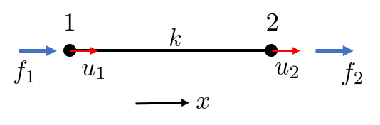
One dimensional rod with two displacements and two forces.

Recall a spring force: $F=k\;x$ , now we apply this on our case

N=k\;\underset{\delta }{\underbrace{\left(u_2 -u_1 \right)} }

where $k=\frac{E\;A}{L}$ . With $N=f_2$ and $f_1 =-N$ we can write

\left\lbrace \begin{array}{ll} f_2 =k\left(u_2 -u_1 \right) & \\ f_1 =k\left(u_1 -u_2 \right) & \end{array}\right.

or on matrix form

k\left\lbrack \begin{array}{cc} 1 & -1\\ -1 & 1 \end{array}\right\rbrack \left\lbrack \begin{array}{c} u_1 \\ u_2 \end{array}\right\rbrack =\left\lbrack \begin{array}{c} f_1 \\ f_2 \end{array}\right\rbrack

\mathbf K_e \mathbf u = \mathbf f

where $\mathbf K_e$ is known as the element stiffness matrix.

Now, consider some arbitrary rod in a two dimensional setting.

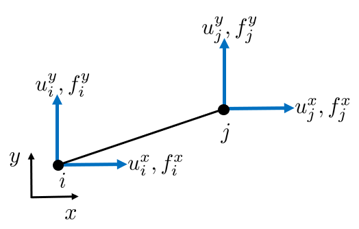
Each node can be translated in the x- and y-direction and each node can carry loads in x- and y-directions.

We shall derive the element stiffness matrix for this rod, but it is easier to first derive it in local coordinates and then transform it into the global coordinates.

Each rod has a local coordinate system $x^{\prime }$ and $y^{\prime }$ and local node numbers $1$ and $2$ . The local coordinate system is rotated compared to the global coordinate system, and the angle is denoted by $\theta$ . In the local coordinates we have

\def\arraystretch{1.5} \left\lbrace \begin{array}{ll} k\left(u_1^{\prime } -u_3^{\prime } \right) & =f_1^{\prime } \\ 0 & =f_2^{\prime } \\ k\left(u_3^{\prime } -u_1^{\prime } \right) & =f_3^{\prime } \\ 0 & =f_4^{\prime } \end{array}\right.

We have zero force normal to the rod since the rod only can carry axial forces. The above relation can be written on matrix form

k\left\lbrack \begin{array}{cccc} 1 & 0 & -1 & 0\\ 0 & 0 & 0 & 0\\ -1 & 0 & 1 & 0\\ 0 & 0 & 0 & 0 \end{array}\right\rbrack \left\lbrack \begin{array}{c} u_1^{\prime } \\ u_2^{\prime } \\ u_3^{\prime } \\ u_4^{\prime } \end{array}\right\rbrack =\left\lbrack \begin{array}{c} f_1^{\prime } \\ f_2^{\prime } \\ f_3^{\prime } \\ f_4^{\prime } \end{array}\right\rbrack

\mathbf K^\prime_e \mathbf u^\prime_e = \mathbf f^\prime_e

known as the local element stiffness matrix.

The transformation matrix

We need a way to transform $\mathbf u^\prime_e$ to $u_i$ and $u_j$ . In other words, we need a relation between $\mathbf u^\prime_e$ and $u_i$ and $u_j$

\def\arraystretch{1.4} \left\lbrace \begin{array}{ll} u_i^x =u_1^{\prime } \cos \theta -u_2^{\prime } \sin \theta & \\ u_i^y =u_1^{\prime } \sin \theta +u_2^{\prime } \cos \theta & \\ u_j^x =u_3^{\prime } \cos \theta -u_4^{\prime } \sin \theta & \\ u_j^y =u_3^{\prime } \sin \theta +u_4^{\prime } \cos \theta & \end{array}\right.

which on matrix form is

\def\arraystretch{1.4} \left\lbrack \begin{array}{c} u_i^x \\ u_i^y \\ u_j^x \\ u_j^y \end{array}\right\rbrack =\left\lbrack \begin{array}{cccc} \cos \theta & -\sin \theta & 0 & 0\\ \sin \theta & \cos \theta & 0 & 0\\ 0 & 0 & \cos \theta & -\sin \theta \\ 0 & 0 & \sin \theta & \cos \theta \end{array}\right\rbrack \left\lbrack \begin{array}{c} u_1^{\prime } \\ u_2^{\prime } \\ u_3^{\prime } \\ u_4^{\prime } \end{array}\right\rbrack

\mathbf u_e = \mathbf L^T \mathbf u^\prime_e

where $\mathbf L^T$ is known as the transformation matrix, and we recognize the rotation matrix within. The transformation matrix has interesting properties: $\mathbf L^T \mathbf L = \mathbf L \mathbf L^T = \mathbf I$ and $\mathbf L^{-1} = \mathbf L^T$ .

Using the transformation matrix we can transform local quantities to global

\mathbf u^\prime_e = \mathbf L^T \mathbf u^\prime_e \Leftrightarrow \mathbf u^\prime_e = \mathbf L \mathbf u_e

\mathbf f_e = \mathbf L^T \mathbf f^\prime_e \Leftrightarrow \mathbf f^\prime_e = \mathbf L \mathbf f_e

Insert (11) and (12) into (7)

\mathbf L^T \mathbf K^\prime_e \mathbf L \mathbf u_e = \mathbf f_e

\boxed{ \mathbf S_e \mathbf u_e = \mathbf f_e }

where $\mathbf S_e$ is known as the element stiffness matrix.

How to compute the transformation matrix $\mathbf L^T$

One could determine the angle $\theta$ . But there is a cheaper way. Let $\mathit{\mathbf{r} }$ define the rod vector such that

\mathbf{r} = \mathbf{p}_j - \mathbf{p}_i

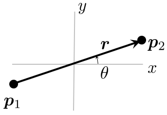
then the normalized vector

\widehat{\mathbf r} =\dfrac{\mathit{\mathbf{r} } }{|\mathit{\mathbf{r} }|}=\left\lbrack \begin{array}{c} \cos \theta \\ \sin \theta \end{array}\right\rbrack =:\left\lbrack \begin{array}{c} c\\ s \end{array}\right\rbrack

such that we get

{\mathit{\mathbf{L} } }^T =\left\lbrack \begin{array}{cccc} c & -s & 0 & 0\\ s & c & 0 & 0\\ 0 & 0 & c & -s\\ 0 & 0 & s & c \end{array}\right\rbrack

and

\mathbf S_e = k\left\lbrack \begin{array}{cccc} c^2 & c\;s & -c^2 & -c\;s\\ c\;s & s^2 & -c\;s & -s^2 \\ -c^2 & -c\;s & c^2 & c\;s\\ c\;s & -s^2 & c\;s & s^2 \end{array}\right\rbrack

We note that the element stiffness matrix is symmetric.

Does it matter how the rod vector is defined? The vector can be defined either by $\mathbf r = \mathbf p_2 - \mathbf p_1$ or $-\mathbf r = \mathbf p_1 - \mathbf p_2$ and we get two situations.

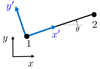
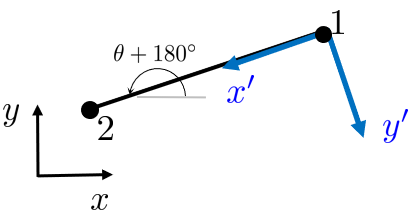
It turns out (which is easily verifiable) that $\mathbf S_e$ is independent of the how the rod vector (or angle $\theta$ ) is defined, i.e., both alternatives yield the same result.

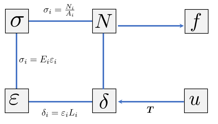
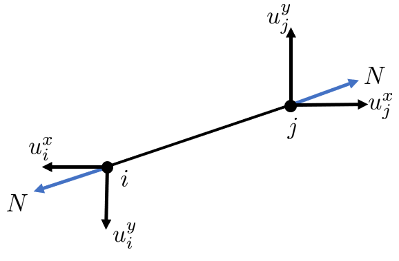
Rod forces, deformations, strains and stresses

The deformation of the rod is given by

\def\arraystretch{1.5} \begin{array}{l} \delta =\Delta u=\left(u_j^x \cos \theta +u_j^y \sin \theta \right)-\left(u_i^x \cos \theta +u_i^y \sin \theta \right)\\ \;\\ \delta =\underset{\mathit{\mathbf{T} } }{\underbrace{\left\lbrack \begin{array}{cccc} -c & -s & c & s \end{array}\right\rbrack } } \left\lbrack \begin{array}{c} u_i^x \\ u_i^y \\ u_j^x \\ u_j^y \end{array}\right\rbrack =\mathit{\mathbf{T} }\cdot \mathbf u_e \end{array}

where $\mathit{\mathbf{T} }$ is called the transformation vector.

We have the rod element rod force

N=\dfrac{EA}{L}\delta =k\;\mathit{\mathbf{T} }\cdot \mathbf u_e

and the element load vector (or reaction forces)

\def\arraystretch{1.5} \begin{array}{l} {\mathit{\mathbf{f} } }^e ={\mathit{\mathbf{T} } }^T N=k\;{\mathit{\mathbf{T} } }_{4\times 1}^T {\mathit{\mathbf{T} } }_{1\times 4} {\;\mathit{\mathbf{u} } }_{4\times 1}^e =k\left\lbrack \begin{array}{c} -c\\ -s\\ c\\ s \end{array}\right\rbrack \left\lbrack \begin{array}{cccc} -c & -s & c & s \end{array}\right\rbrack \left\lbrack \begin{array}{c} u_i^x \\ u_i^y \\ u_j^x \\ u_j^y \end{array}\right\rbrack \\ \;\\ \left\lbrack \begin{array}{c} f_i^x \\ f_i^y \\ f_j^x \\ f_j^y \end{array}\right\rbrack =\underset{ \mathbf{S}_e }{\underbrace{\dfrac{EA}{L}\left\lbrack \begin{array}{cccc} c^2 & c\;s & -c^2 & -c\;s\\ c\;s & s^2 & -c\;s & -s^2 \\ -c^2 & -c\;s & c^2 & c\;s\\ c\;s & -s^2 & c\;s & s^2 \end{array}\right\rbrack } } \left\lbrack \begin{array}{c} u_i^x \\ u_i^y \\ u_j^x \\ u_j^y \end{array}\right\rbrack \end{array}

The element strain is obtained by

\varepsilon =\dfrac{\delta }{L}

and the stress by

\sigma =\dfrac{N}{A}

note that the length of the element can be easily computed by

L=|\mathit{\mathbf{r} }|=|{\mathit{\mathbf{p} } }_2 -{\mathit{\mathbf{p} } }_1 |

Complete Truss solver - Matlab implementation

Let us analyze a structure as an example and look at the implementation details in Matlab.

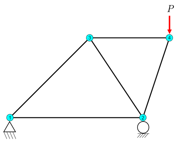
The structure is loaded by a force $P$ with the topology given by

P = [0 0
     5 0
     3 3
     6 3]*100; % mm
edges = [1 2
         1 3
         2 3
         2 4
         3 4];

Problem statement:

Given the structure above, determine all displacements, member forces, deformations, strains and stresses as well as reaction forces in the supports.

Solution

The coordinates are given by the variables P and the edges define the node connectivity.

\textrm{nodes}=\left\lbrack \begin{array}{cc} 1 & 2\\ 1 & 3\\ 2 & 3\\ 2 & 4\\ 3 & 4 \end{array}\right\rbrack \overset{\textrm{Element} }{\begin{array}{c} 1\\ 2\\ 3\\ 4\\ 5 \end{array} }

The order of the columns in nodes is not important.

Using the topological data from above, we can visualize the truss structure in Matlab as follows:

figure
hold on
patch('Faces',edges,'Vertices',P,'LineWidth',2)
plot(P(:,1),P(:,2),'ok','MarkerFaceColor','c','MarkerSize',14)
nnod = size(P,1);
text(P(:,1)-0.05,P(:,2),cellstr(num2str([1:nnod]')))
axis equal
axis off
for i=1:5
    inod = edges(i,:);
    xm = mean(P(inod,1));
    ym = mean(P(inod,2));
    text(xm,ym,num2str(i),'backgroundColor','y')
end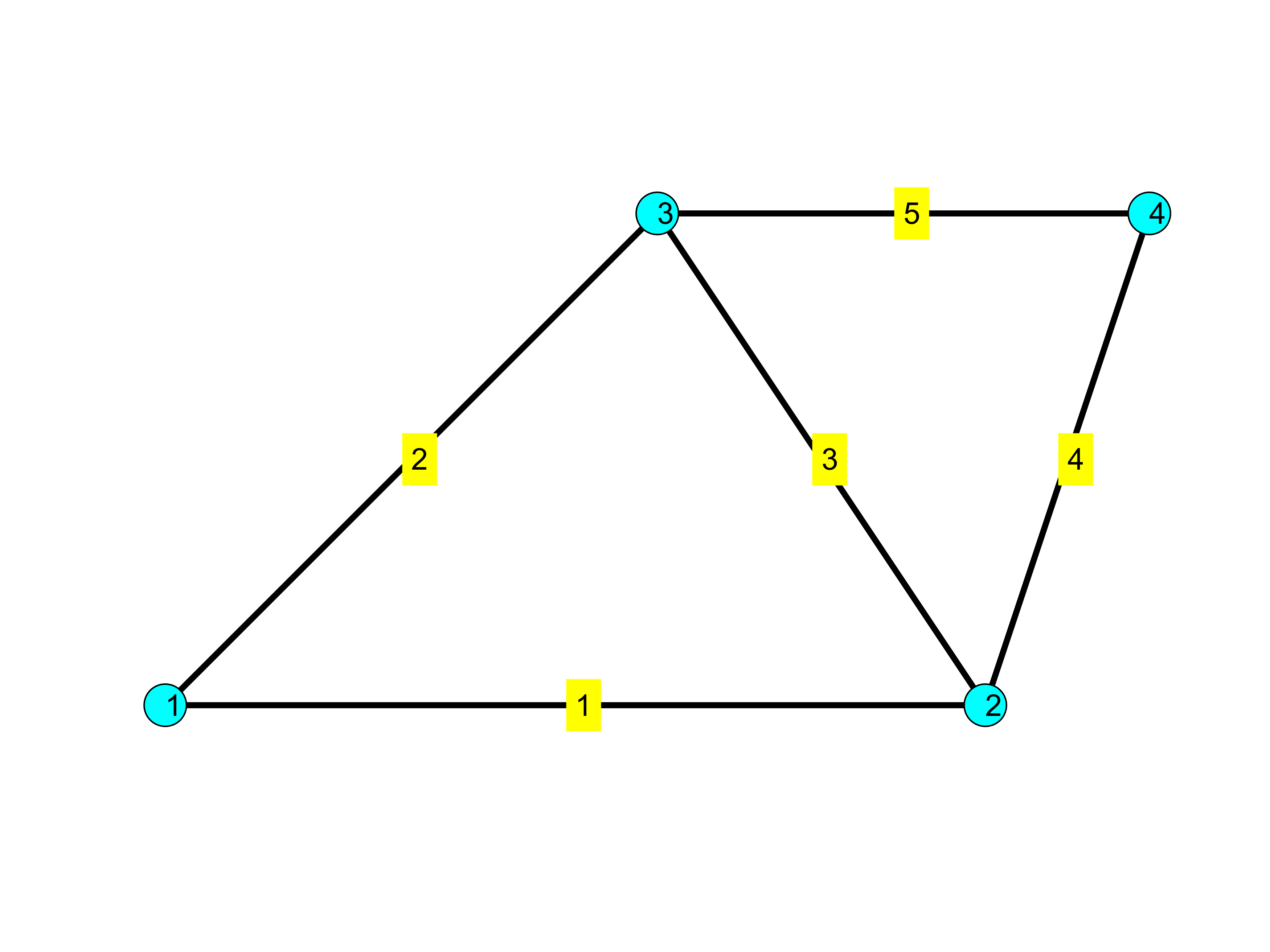

The total number of degrees of freedom (or equations), $n_\textrm{dof}$ is given by

n_\textrm{dof} = n_\textrm{nod} \cdot n_\textrm{loc} = 4\cdot 2 = 8

where $n_\textrm{nod}$ is the number of nodes and $n_\textrm{loc}$ is the number of local degrees of freedom per node.

The global displacement field and load field are given by

\mathit{\mathbf{u} }=\left\lbrack \begin{array}{c} u_1^x =0\\ u_1^y =0\\ u_2^x \\ u_2^y =0\\ u_3^x \\ u_3^y \\ u_4^x \\ u_4^y \end{array}\right\rbrack ,\mathit{\mathbf{f} }=\left\lbrack \begin{array}{c} f_1^x =0\\ f_1^y =0\\ f_2^x =0\\ f_2^y =0\\ f_3^x =0\\ f_3^y =0\\ f_4^x =0\\ f_4^y =-P \end{array}\right\rbrack

With the resulting linear system taking the form of

{\mathit{\mathbf{S} } }_{8\times 8} {\;\mathit{\mathbf{u} } }_{8\times 1} ={\mathit{\mathbf{f} } }_{8\times 1}

The unknown displacements are computed by establishing the global stiffness matrix (system matrix) $\mathbf S$ . Creating the linear system (28) and solving for $\mathbf u$ . This is done by the following steps:

Initialize the stiffness matrix, i.e., set it to zero, $\mathbf S = \mathbf 0$ .
Loop over all elements, and for each element:
Compute the element stiffness matrix, $\mathbf S_e$
Add the element stiffness matrix into the global stiffness matrix
Add the element load vector to the global load vector
Apply boundary conditions
Solve the linear system

We begin with some preliminaries and initialize the global system matrix and vectors using the number of degrees of freedom.

nele = 5

nnod = 4

dofs = 8

S = zeros(dofs, dofs);
f = zeros(dofs,1);
u = f;

Sprim = [1  0 -1  0
         0  0  0  0
         -1 0  1  0
         0  0  0  0];
Ltot = 0; %Total length of the structure.
E = 210000*ones(nele,1);    % Young's modulus
A = 4*6*ones(nele,1);    % Cross sectional area

Element 1

We begin by computing which global degrees of freedom correspond to our first element.

inod = 1x2    
     1     2

The node numbers correspond to degrees of freedom, for our problem we have two, i.e., $x-$ and $y-$ translation. The data structure of ieqs is the same as for the displacements and loads above.

ieqs = 1x4    
     1     0     3     0

ieqs = 1x4    
     1     2     3     4

Computing the element stiffness matrix

p1 = 1x2    
     0     0

p2 = 1x2    
   500     0

r = 1x2    
   500     0

L = 500

Ltot = 500

er = 1x2    
     1     0

LT = 4x4    
     1     0     0     0
     0     1     0     0
     0     0     1     0
     0     0     0     1

k = 10080

Se = 4x4    
       10080           0      -10080           0
           0           0           0           0
      -10080           0       10080           0
           0           0           0           0

Assembly process

The element stiffness matrix $\mathbf S_e$ needs to be added to the global stiffness matrix $\mathbf S$ . We need to ensure that the correct components from the element matrix are mapped to the corresponding components of the global stiffness matrix. This is done using the previously computed list of degrees of freedom, stored in the variable ieqs. We append (add) the stiffness contributions using

S = 8x8    
       10080           0      -10080           0           0           0           0           0
           0           0           0           0           0           0           0           0
      -10080           0       10080           0           0           0           0           0
           0           0           0           0           0           0           0           0
           0           0           0           0           0           0           0           0
           0           0           0           0           0           0           0           0
           0           0           0           0           0           0           0           0
           0           0           0           0           0           0           0           0

This is the simplest form of assembly in code. It is easy to read and understand. It is however not very efficient for very large problems with hundreds of thousands of elements. So there exists other methods of dealing with this. But that is a topic for a course in high performance computing.

The rest of the elements are dealt with in an automated manner by executing the above lines of code for each element number, iel. This is done using the for loop:

iel = 2
L = 424.2641
Ltot = 924.2641
er = 1x2    
    0.7071    0.7071

k = 1.1879e+04
Se = 4x4    
1.0e+03 *

    5.9397    5.9397   -5.9397   -5.9397
    5.9397    5.9397   -5.9397   -5.9397
   -5.9397   -5.9397    5.9397    5.9397
   -5.9397   -5.9397    5.9397    5.9397

S = 8x8    
1.0e+04 *

    1.6020    0.5940   -1.0080         0   -0.5940   -0.5940         0         0
    0.5940    0.5940         0         0   -0.5940   -0.5940         0         0
   -1.0080         0    1.0080         0         0         0         0         0
         0         0         0         0         0         0         0         0
   -0.5940   -0.5940         0         0    0.5940    0.5940         0         0
   -0.5940   -0.5940         0         0    0.5940    0.5940         0         0
         0         0         0         0         0         0         0         0
         0         0         0         0         0         0         0         0

iel = 3
L = 360.5551
Ltot = 1.2848e+03
er = 1x2    
   -0.5547    0.8321

k = 1.3978e+04
Se = 4x4    
1.0e+03 *

    4.3011   -6.4516   -4.3011    6.4516
   -6.4516    9.6774    6.4516   -9.6774
   -4.3011    6.4516    4.3011   -6.4516
    6.4516   -9.6774   -6.4516    9.6774

S = 8x8    
1.0e+04 *

    1.6020    0.5940   -1.0080         0   -0.5940   -0.5940         0         0
    0.5940    0.5940         0         0   -0.5940   -0.5940         0         0
   -1.0080         0    1.4381   -0.6452   -0.4301    0.6452         0         0
         0         0   -0.6452    0.9677    0.6452   -0.9677         0         0
   -0.5940   -0.5940   -0.4301    0.6452    1.0241   -0.0512         0         0
   -0.5940   -0.5940    0.6452   -0.9677   -0.0512    1.5617         0         0
         0         0         0         0         0         0         0         0
         0         0         0         0         0         0         0         0

iel = 4
L = 316.2278
Ltot = 1.6010e+03
er = 1x2    
    0.3162    0.9487

k = 1.5938e+04
Se = 4x4    
1.0e+04 *

    0.1594    0.4781   -0.1594   -0.4781
    0.4781    1.4344   -0.4781   -1.4344
   -0.1594   -0.4781    0.1594    0.4781
   -0.4781   -1.4344    0.4781    1.4344

S = 8x8    
1.0e+04 *

    1.6020    0.5940   -1.0080         0   -0.5940   -0.5940         0         0
    0.5940    0.5940         0         0   -0.5940   -0.5940         0         0
   -1.0080         0    1.5975   -0.1670   -0.4301    0.6452   -0.1594   -0.4781
         0         0   -0.1670    2.4021    0.6452   -0.9677   -0.4781   -1.4344
   -0.5940   -0.5940   -0.4301    0.6452    1.0241   -0.0512         0         0
   -0.5940   -0.5940    0.6452   -0.9677   -0.0512    1.5617         0         0
         0         0   -0.1594   -0.4781         0         0    0.1594    0.4781
         0         0   -0.4781   -1.4344         0         0    0.4781    1.4344

iel = 5
L = 300
Ltot = 1.9010e+03
er = 1x2    
     1     0

k = 16800
Se = 4x4    
       16800           0      -16800           0
           0           0           0           0
      -16800           0       16800           0
           0           0           0           0

S = 8x8    
1.0e+04 *

    1.6020    0.5940   -1.0080         0   -0.5940   -0.5940         0         0
    0.5940    0.5940         0         0   -0.5940   -0.5940         0         0
   -1.0080         0    1.5975   -0.1670   -0.4301    0.6452   -0.1594   -0.4781
         0         0   -0.1670    2.4021    0.6452   -0.9677   -0.4781   -1.4344
   -0.5940   -0.5940   -0.4301    0.6452    2.7041   -0.0512   -1.6800         0
   -0.5940   -0.5940    0.6452   -0.9677   -0.0512    1.5617         0         0
         0         0   -0.1594   -0.4781   -1.6800         0    1.8394    0.4781
         0         0   -0.4781   -1.4344         0         0    0.4781    1.4344

The resulting system $\mathbf S \mathbf u = \mathbf f$ , however, is singular. In mechanical terms, it contains rigid body motions. In mathematical terms, it has an infinite amount of solutions. To alleviate these rigid body motions, we need to clamp down the mechanical system by introducing boundary conditions which pose enough constraints on the displacements such that rigid body motions are prohibited. This is done for instance by eliminating equations, i.e., rows and columns corresponding to the degrees of freedom where the displacements are known. Solving the reduced system gives a unique solution.

Note that special treatment of the right-hand side is required in cases where the displacements are non-zero. See the section on Truss Analysis for details.

We assign the known boundary conditions and loads.

presc = [1 2 4];     % prescribed degrees of freedom
u(presc) = 0;
f(2*4) = -10000;     % a single load at node 4 in the y-direction

free = setdiff(1:dofs, presc); % Free DOFs

u(free) = S(free,free)\f(free) % Solving the system

We can separate the x- and y-components of the displacements into a two column matrix for easier handling in the visualization step below.

U = 4x2    
         0         0
   -0.1984         0
    0.2467    0.0901
    0.4451   -0.9116

We can also compute the resultant of the nodal displacement since it usually is of interest when evaluating requirements. We do this be computing the 2-norm of each row of the matrix (using the vectorized approach of course).

Total displacements in each node.

Visualize displacements

figure
hold on
patch('Faces',edges,'Vertices',P,'LineWidth',2)
patch('Faces',edges,'Vertices',P+U*80,'LineWidth',1,'LineStyle',':')
axis equal
axis off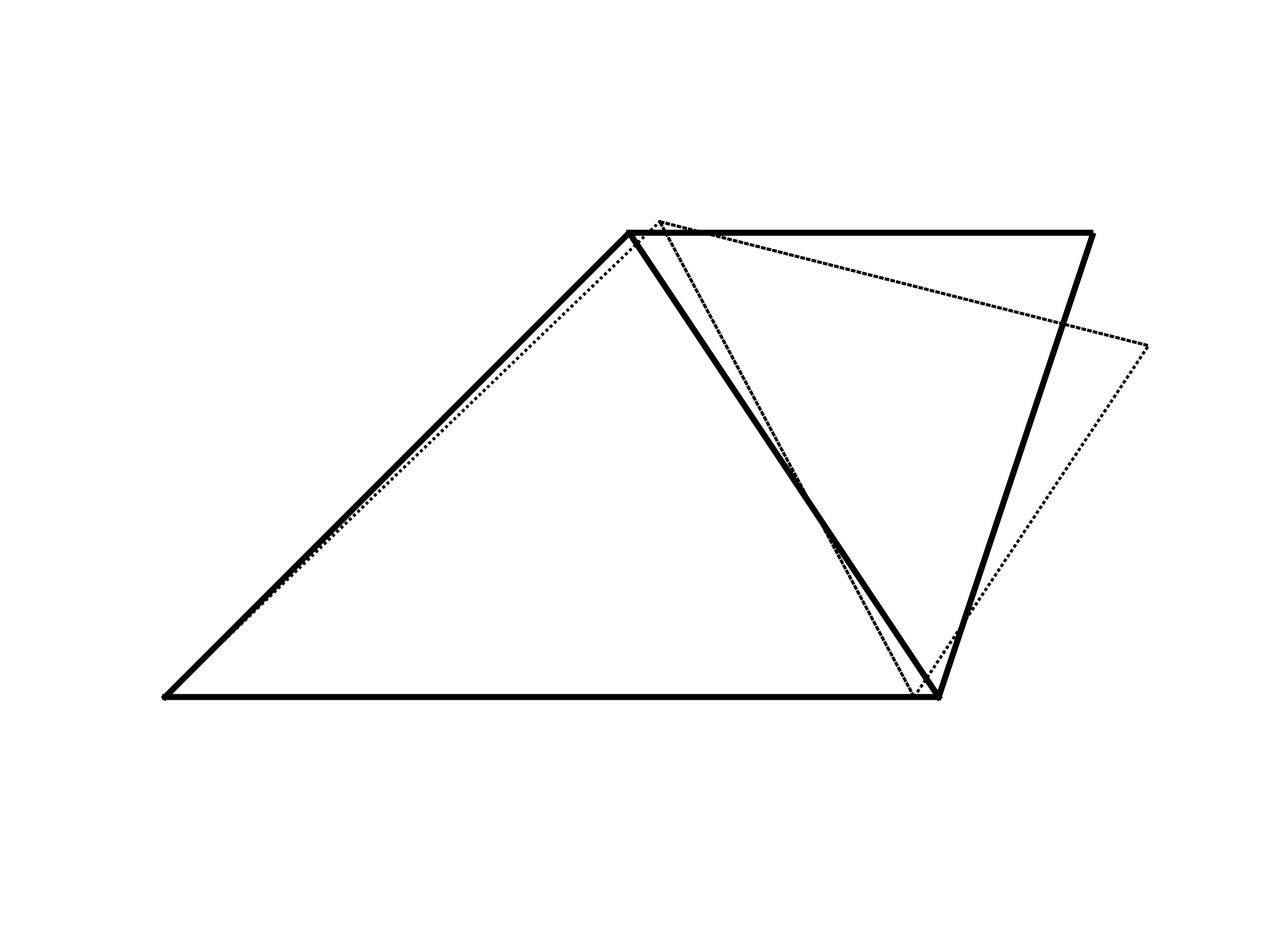

The generated displacement field (dashed line) is scaled up by a factor of 80 since the displacements are otherwise too small to see.

Computing rod quantities

Once the displacements have been computed we can compute the normal forces, resultant forces, deformations, strains and stresses.

React = zeros(dofs,1); % Reaction forces
delta = zeros(nele,1); % Deformation vector
N = delta;             % Force vector
epsilon = delta;       % Strain vector
sigma = delta;         % Stress vector

for iel = 1:nele
    inod = edges(iel,:);
    ieqs = zeros(1,4); %[0 0 0 0]
    ieqs(1:2:end) = inod*2-1;
    ieqs(2:2:end) = inod*2;
    iu = u(ieqs); % element displacements

    p1 = P(inod(1), :);
    p2 = P(inod(2), :);
    r = p2-p1;
    L = norm(r); % length of the bar
    er = r/L; % direction, unit vector
    c = er(1);
    s = er(2);
    T = [-c -s c s];
    
    iA = A(iel);   % element area
    iE = E(iel);   % element Young's modulus
    k = (iA*iE/L); % element stiffness

    idelta = T*iu;   % element deformation
    iN = k * idelta; % element force
    fe = T'*iN;      % nodal force
    iepsilon = idelta/L; % element strain
    isigma = iN/iA;      % element stress

    React(ieqs) = React(ieqs) + fe; % Add up all reaction forces
    N(iel) = iN;
    delta(iel) = idelta;
    epsilon(iel) = iepsilon;
    sigma(iel) = isigma;
end
React = [React(1:2:end), React(2:2:end)] % Reaction forces split into x and y components

React = 4x2    
1.0e+04 *

    0.0000   -0.2000
   -0.0000    1.2000
    0.0000   -0.0000
   -0.0000   -1.0000

Once the quantities of interest are computed, we will visualize them on the deformed structure. Since the displacements are typically very small, we will scale up the deformation in order to see a trend.

The quantities will be shown using a color field for a fast overview, but we will also add text boxes to give numerical values for more accurate reading.

scale = 80;
X = P(:,1); Y = P(:,2); Ux = U(:,1); Uy = U(:,2);
Xm = mean(X(edges')+Ux(edges')*scale,1);
Ym = mean(Y(edges')+Uy(edges')*scale,1);

figure; hold on
patch('Faces',edges,'Vertices',P,'EdgeAlpha',0.1)
patch(X(edges')+Ux(edges')*scale,Y(edges')+Uy(edges')*scale,[sigma,sigma]','EdgeColor','flat', 'LineWidth',2)
axis equal
colormap jet; colorbar
text(Xm,Ym,cellstr(num2str(sigma)),'BackgroundColor','w')
title('Member stresses [MPa]')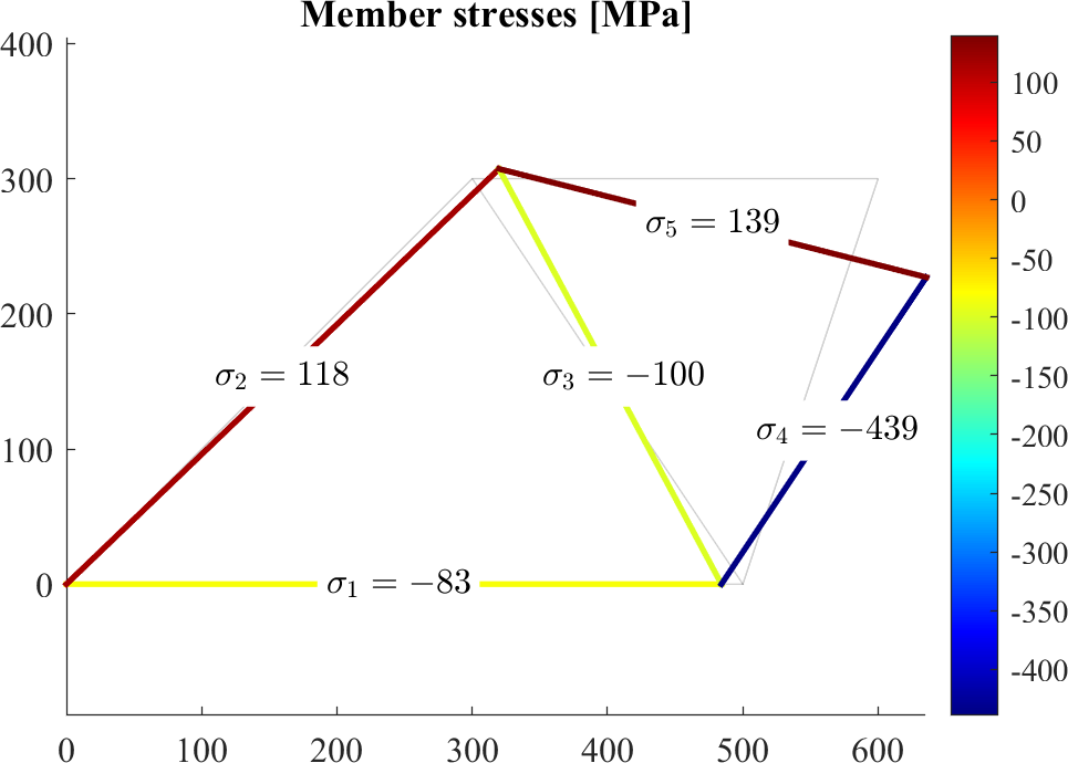

figure; hold on
patch('Faces',edges,'Vertices',P,'EdgeAlpha',0.1)
patch(X(edges')+Ux(edges')*scale,Y(edges')+Uy(edges')*scale,[N,N]','EdgeColor','flat', 'LineWidth',2)
axis equal
colormap jet; colorbar
text(Xm,Ym,cellstr(num2str(N)),'BackgroundColor','w')
title('Member forces [N]')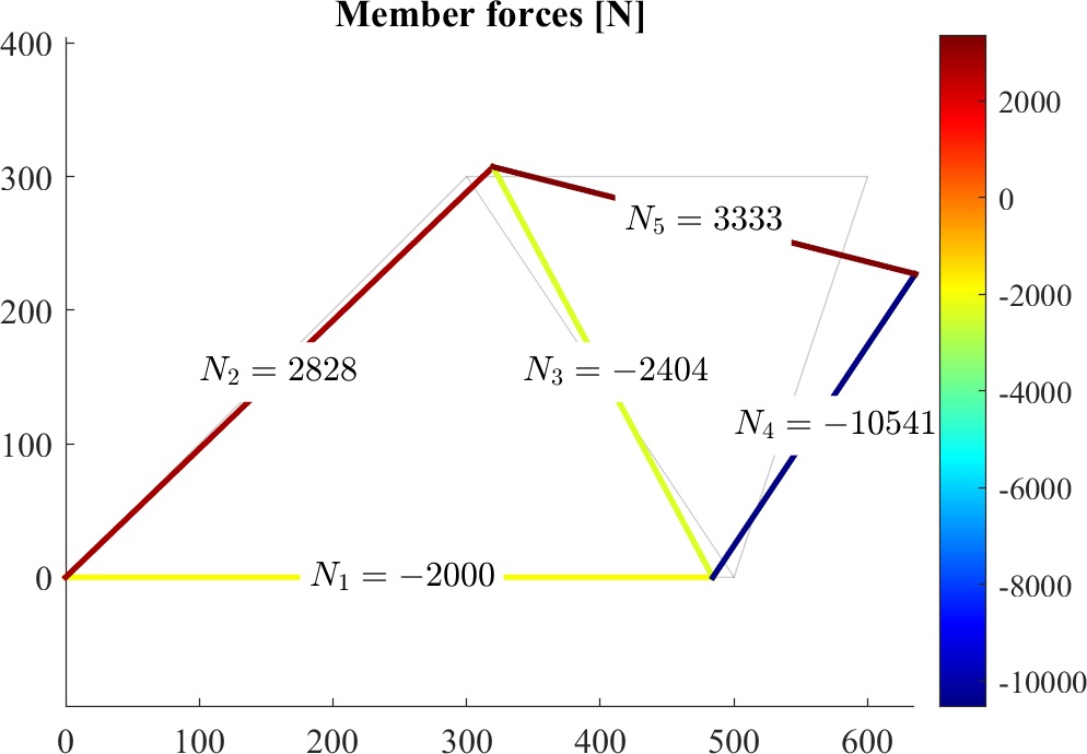

figure; hold on
patch('Faces',edges,'Vertices',P,'EdgeAlpha',0.1)
patch(X(edges')+Ux(edges')*scale,Y(edges')+Uy(edges')*scale,[delta,delta]','EdgeColor','flat', 'LineWidth',2)
axis equal
colormap jet; colorbar
text(Xm,Ym,cellstr(num2str(delta)),'BackgroundColor','w')
title('Member deformations [mm]')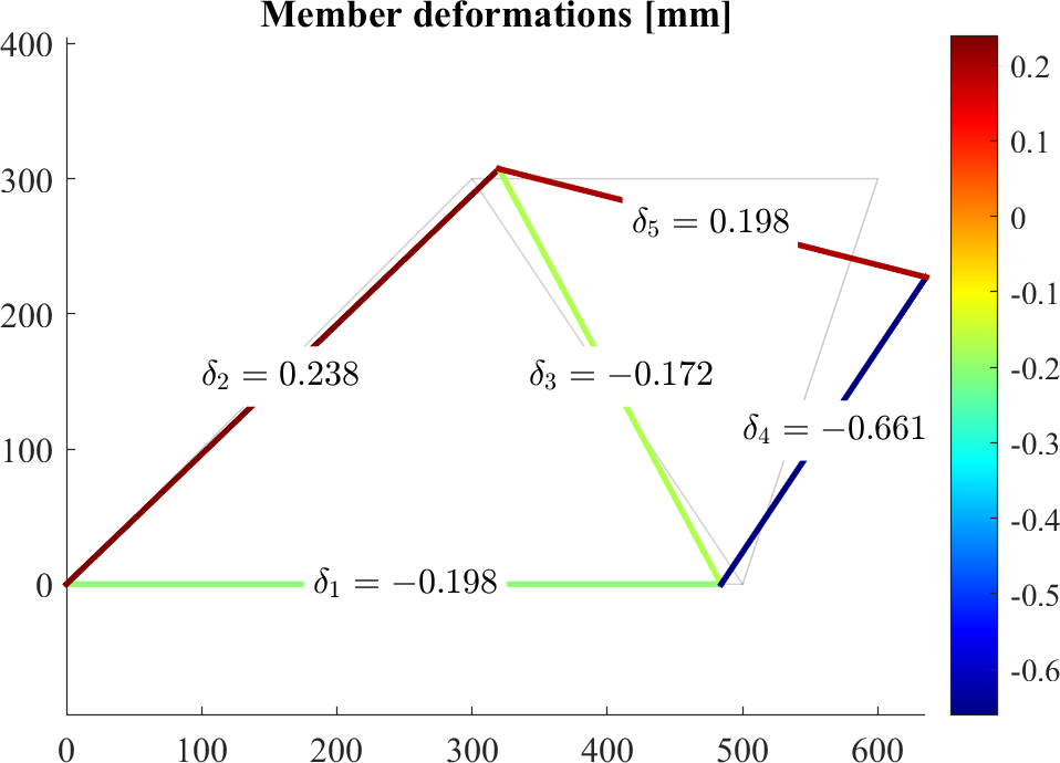

figure; hold on
patch('Faces',edges,'Vertices',P,'EdgeAlpha',0.1)
patch(X(edges')+Ux(edges')*scale,Y(edges')+Uy(edges')*scale,[epsilon,epsilon]','EdgeColor','flat', 'LineWidth',2)
axis equal
colormap jet; colorbar
text(Xm,Ym,cellstr(num2str(epsilon)),'BackgroundColor','w')
title('Member strains [mm/mm]')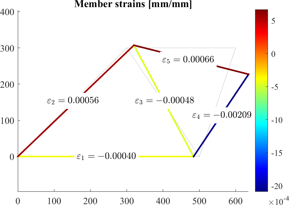

Example - Prescribed displacements

Here, in addition for nodal forces, we also have nodes with prescribed displacements which are non-zero. This is the same as deforming a spring to a certain length, it will correspond to a force, but we control the displacement instead.

$\delta =1$ mm. $P=10$ kN.

clear
P = [0 0
     6 0
     4 2
     0 2]*100; % mm
nnod = size(P,1);
edges = [1 2
         3 4
         1 3
         3 2];

Initiate variables

nele = size(edges,1);
nnod = size(P,1);
dofs = nnod*2; %number of degrees of freedom
S = zeros(dofs, dofs);
f = zeros(dofs,1);
u = f;
Sprim = [1 0 -1 0
         0 0  0 0
         -1 0 1 0
         0  0 0 0];
Ltot = 0; % Total length of the structure.

Visualize the structure

figure; hold on
patch('Faces',edges,'Vertices',P,'LineWidth',2, 'HandleVisibility','off')
dx = max(P(:,1))-min(P(:,1));
dy = max(P(:,2))-min(P(:,2));
plot(P(:,1),P(:,2),'ok','MarkerFaceColor','k','MarkerSize',14, 'HandleVisibility','off')
text(P(:,1)-0.01*dx,P(:,2),cellstr(num2str([1:nnod]')),'Color','w', 'HandleVisibility','off');
axis equal
axis off
for i=1:nele
    inod = edges(i,:);
    xm = mean(P(inod,1));
    ym = mean(P(inod,2));
    text(xm,ym,num2str(i),'backgroundColor','y')
end

User defined parameters

E = 210000*ones(nele,1);    % Young's modulus
A = 4*6*ones(nele,1);    % Cross sectional area

presc = [1 2 3 7 8];     % prescribed degrees of freedom
u(presc) = [0, 0, 2, 0, 0]; %mm
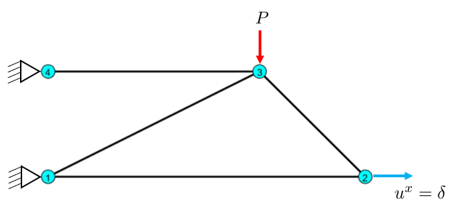
f(3*2) = -10000;

free = setdiff(1:dofs, presc); % Free DOFs

Visualize the Load case

To visually verify load case and boundary conditions

px = presc(mod(presc,2)==1);
xinds = (px+1)/2;
py = presc(mod(presc,2)==0);
yinds = py/2;
Fx = f(1:2:end); Fy = f(2:2:end);
dd = sqrt(dx^2+dy^2);
quiver(P(:,1)+sign(Fx)*dd*0.03,P(:,2),Fx,zeros(nnod,1),0.08,'Color','r','LineWidth',2,'DisplayName','f_x')
quiver(P(:,1),P(:,2)+sign(Fy)*dd*0.03,zeros(nnod,1),Fy,0.08,'Color','b','LineWidth',2,'DisplayName','f_y')
plot(P(xinds,1),P(xinds,2),'sk','MarkerFaceColor','r','MarkerSize',25,'DisplayName','u_x');
plot(P(yinds,1),P(yinds,2),'dk','MarkerFaceColor','b','MarkerSize',14,'DisplayName','u_y');
text(P(:,1)-0.01*dx,P(:,2),cellstr(num2str([1:nnod]')),'Color','w','HandleVisibility','off');
legend show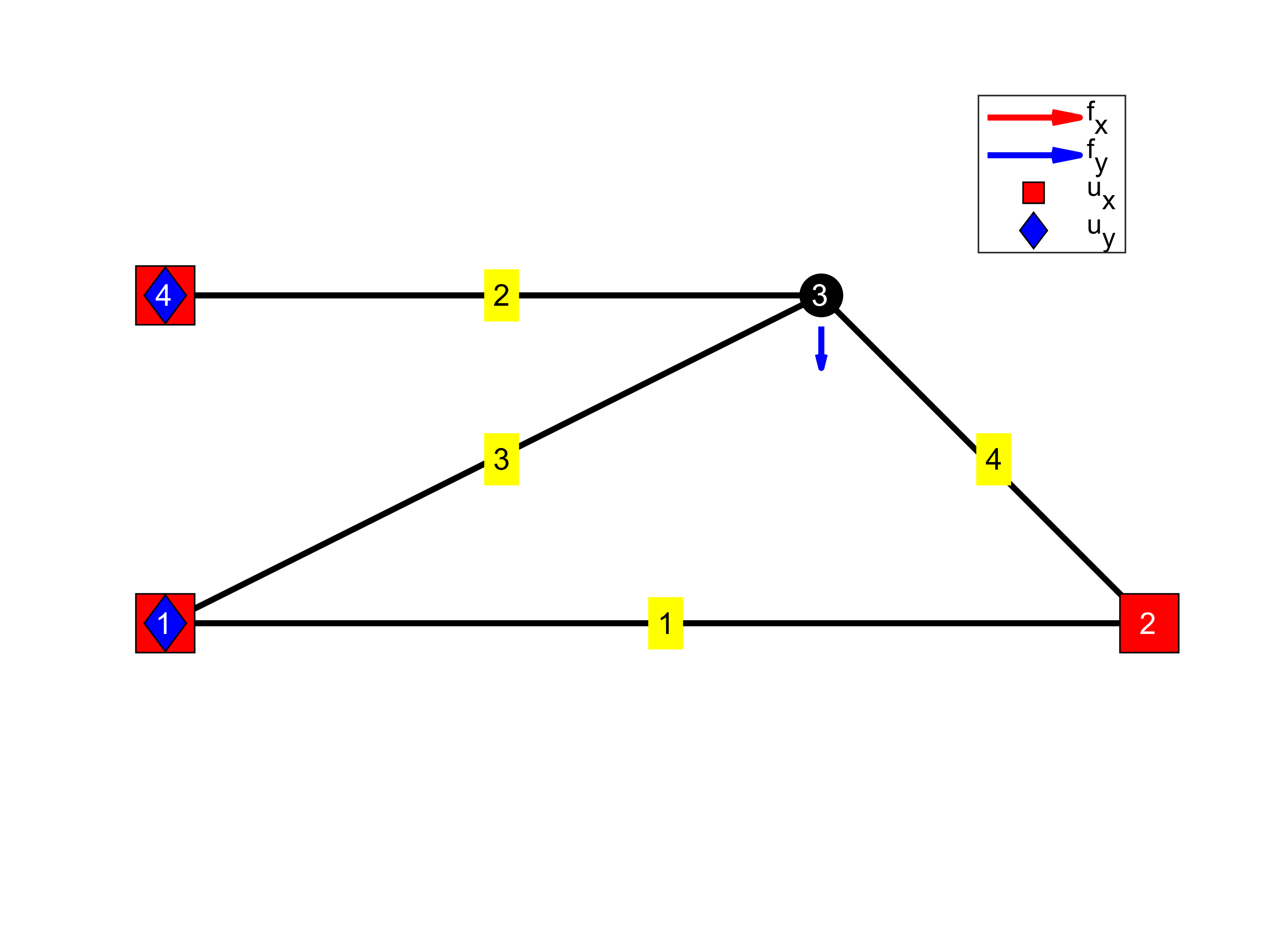

Computing the stiffness matrix

for iel = 1:nele
    inod = edges(iel,:);
    ieqs = zeros(1,4); %[0 0 0 0]
    ieqs(1:2:end) = inod*2-1;
    ieqs(2:2:end) = inod*2;
    p1 = P(inod(1), :);
    p2 = P(inod(2), :);
    r = p2-p1;
    L = norm(r); % length of the bar
    Ltot = Ltot + L;
    er = r/L; % direction, unit vector
    c = er(1);
    s = er(2);
    R = [c -s
         s  c];
    % Transformation matrix
    LT = [R, zeros(2);
         zeros(2), R];
    % Element stiffness matrix
    iA = A(iel);  % element area
    iE = E(iel);  % element Young's modulus
    k = (iA*iE/L); % element stiffness
    Se  = k * LT*Sprim*LT';
    S(ieqs,ieqs) = S(ieqs,ieqs) + Se ;
end

Now we deal with the prescribed displacements.

u(free) = S(free,free)\f(free);
U = [u(1:2:end), u(2:2:end)]

U = 4x2    
         0         0
    2.0000   -7.1985
    1.5873   -7.6112
         0         0

UR = sum(U.^2,2).^0.5 % Resultant displacement

Visualize the displacements

scale = 5;
figure
hold on
patch('Faces',edges,'Vertices',P,'LineWidth',2)
patch('Faces',edges,'Vertices',P+U*scale,'LineWidth',1,'LineStyle',':')
axis equal
axis off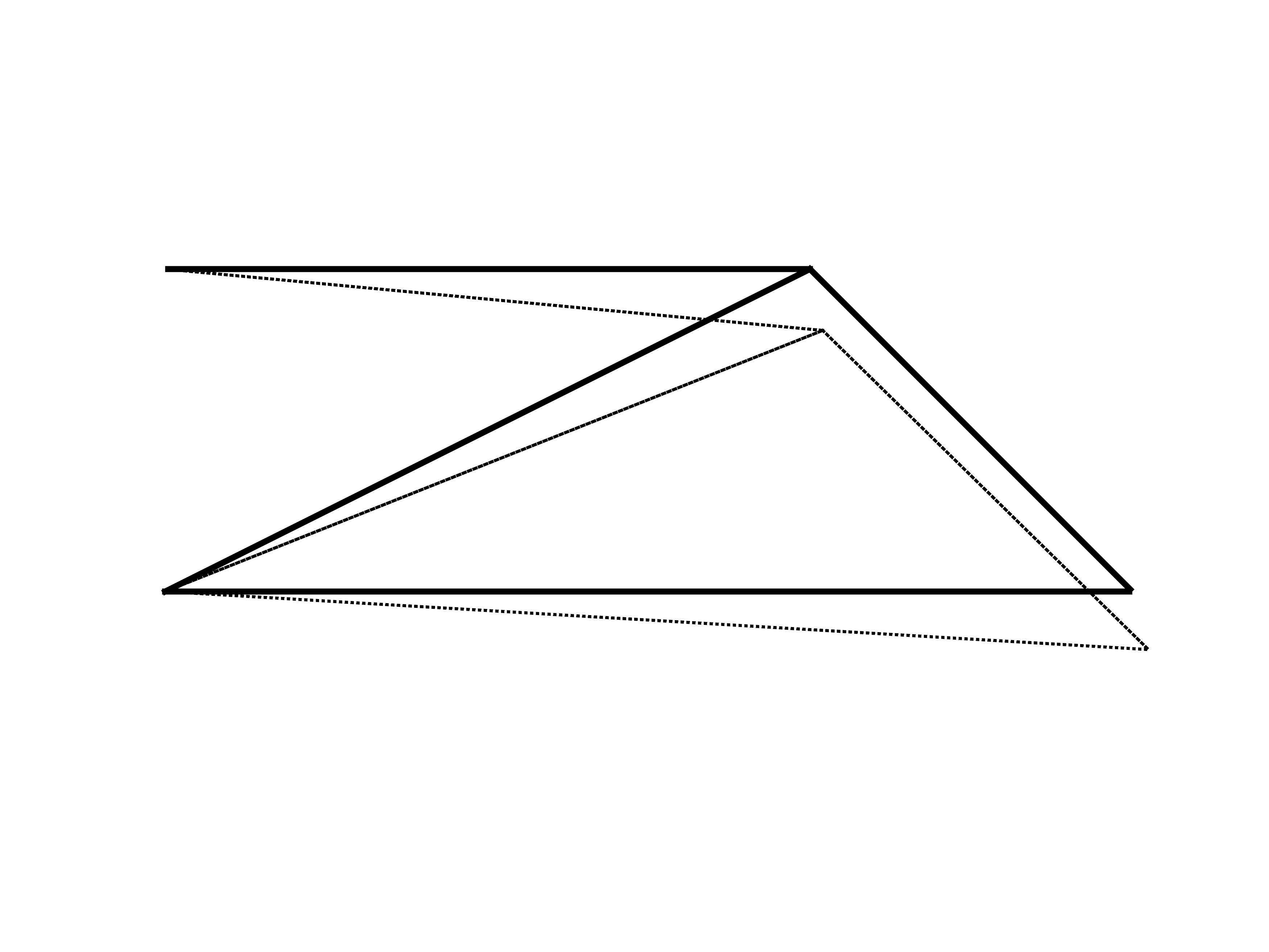

Computing rod quantities

React = zeros(dofs,1);
delta = zeros(nele,1);
N = delta; epsilon = delta; sigma = delta;

for iel = 1:nele
    inod = edges(iel,:);
    ieqs = zeros(1,4); %[0 0 0 0]
    ieqs(1:2:end) = inod*2-1;
    ieqs(2:2:end) = inod*2;
    iu = u(ieqs);

    p1 = P(inod(1), :);
    p2 = P(inod(2), :);
    r = p2-p1;
    L = norm(r); % length of the bar
    er = r/L; % direction, unit vector
    c = er(1);
    s = er(2);
    R = [c -s
         s  c];
    % Transformation matrix
    LT = [R, zeros(2);
         zeros(2), R];
    T = [-c -s c s];
    
    iA = A(iel);   % element area
    iE = E(iel);   % element Young's modulus
    k = (iA*iE/L); % element stiffness

    idelta = T*iu;
    iN = k * idelta;
    fe = T'*iN;
    iepsilon = idelta/L;
    isigma = iN/iA;

    React(ieqs) = React(ieqs) + fe;
    N(iel) = iN;
    delta(iel) = idelta;
    epsilon(iel) = iepsilon;
    sigma(iel) = isigma;
end

The reaction forces in each node.

React = [React(1:2:end), React(2:2:end)]

React = 4x2    
1.0e+04 *

    0.3200    1.0000
    1.6800    0.0000
    0.0000   -1.0000
   -2.0000         0

Visualize color fields

X = P(:,1); Y = P(:,2); Ux = U(:,1); Uy = U(:,2);
Xm = mean(X(edges')+Ux(edges')*scale,1);
Ym = mean(Y(edges')+Uy(edges')*scale,1);

figure; hold on
patch('Faces',edges,'Vertices',P,'EdgeAlpha',0.1)
patch(X(edges')+Ux(edges')*scale,Y(edges')+Uy(edges')*scale,[sigma,sigma]','EdgeColor','flat', 'LineWidth',2)
axis equal
colormap jet; colorbar
for iel=1:nele
    text(Xm(iel),Ym(iel),sprintf('$\\sigma_{%d}=%0.0f$',iel,sigma(iel)),'BackgroundColor','w','Interpreter','latex')
end
title('Member stresses [MPa]')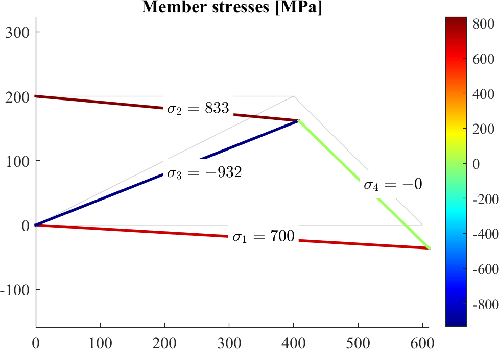

figure; hold on
patch('Faces',edges,'Vertices',P,'EdgeAlpha',0.1)
patch(X(edges')+Ux(edges')*scale,Y(edges')+Uy(edges')*scale,[N,N]','EdgeColor','flat', 'LineWidth',2)
axis equal
colormap jet; colorbar
for iel=1:nele
    text(Xm(iel),Ym(iel),sprintf('$N_{%d}=%0.0f$',iel,N(iel)),'BackgroundColor','w','Interpreter','latex')
end
title('Member forces [N]')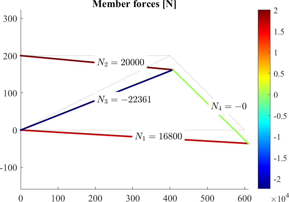

figure; hold on
patch('Faces',edges,'Vertices',P,'EdgeAlpha',0.1)
patch(X(edges')+Ux(edges')*scale,Y(edges')+Uy(edges')*scale,[delta,delta]','EdgeColor','flat', 'LineWidth',2)
axis equal
colormap jet; colorbar
for iel=1:nele
    text(Xm(iel),Ym(iel),sprintf('$\\delta_{%d}=%0.3f$',iel,delta(iel)),'BackgroundColor','w','Interpreter','latex')
end
title('Member deformations [mm]')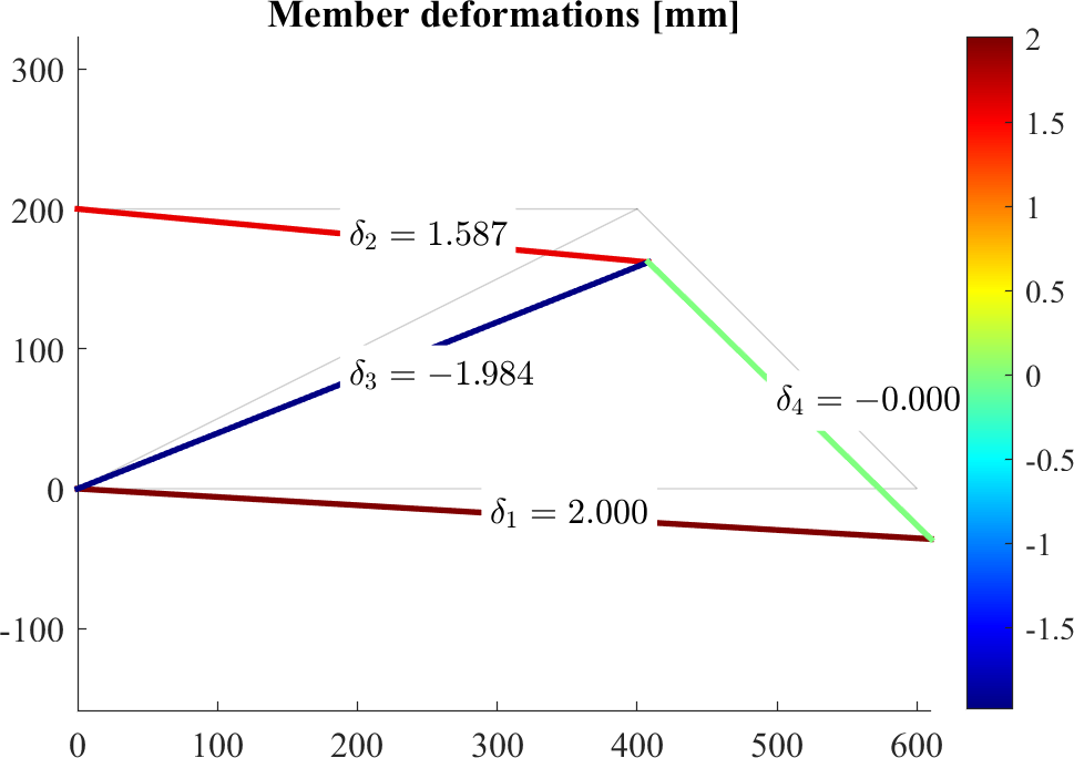

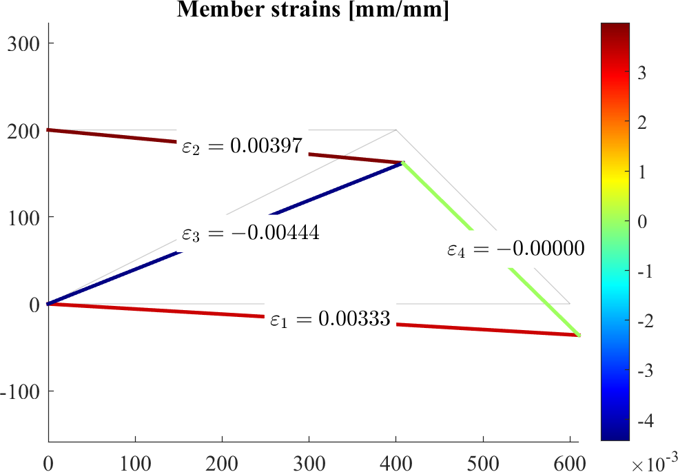
figure; hold on
patch('Faces',edges,'Vertices',P,'EdgeAlpha',0.1)
patch(X(edges')+Ux(edges')*scale,Y(edges')+Uy(edges')*scale,[epsilon,epsilon]','EdgeColor','flat', 'LineWidth',2)
axis equal
colormap jet; colorbar
for iel=1:nele
    text(Xm(iel),Ym(iel),sprintf('$\\varepsilon_{%d}=%0.5f$',iel,epsilon(iel)),'BackgroundColor','w','Interpreter','latex')
end
title('Member strains [mm/mm]')

Applied Mechanics