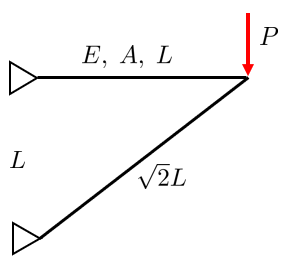
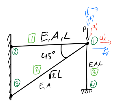
The simple truss is represented by two rods that are attached to each other in the right corner (node) using a pin connector which is assumed to be moment free. The other two ends of the rods are firmly fixed in place, which is denoted by the two triangles. A point force is placed at the node, denoted by P. The rods can only carry axial force, meaning that loads cannot be applied anywhere but at the nodes. This problem is a 2D planar problem, so every node has two degrees of freedom i.e., it can be translated in the x and y-direction.
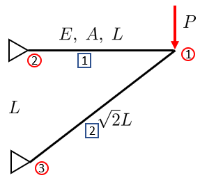
We begin our analysis by numbering each rod and each node. Each rod has four quantities of interest: normal forces, Ni, normal stresses, σi, strains, εi and deformations δi where i=1,2. Additionally each node has two quantities of interest: nodal forces fj and nodal displacements uj where j=1,2,3.
For a structure like this, the interesting questions are:
Is the structure able to carry the load? The the structural requirements are typically posed on the maximum stress and displacements as well as reaction forces, i.e., nodal forces at the boundary conditions.
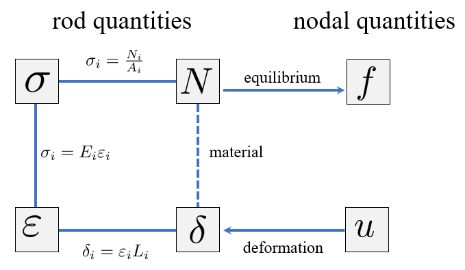
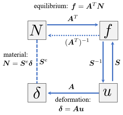
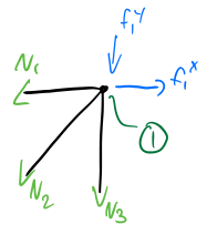
An overview of the relations between nodal quantities and rod quantities is given by the figure below
These relations essentially form the equation
δ=EAFL
which is the simplest solution (setting f=0) to the boundary value problem:
This is why the method in this (and the following) section is also known as the direct approach, since we are tackling the differential equation directly, but also with a loss of generality.
In what follows, we shall derive a method for determining the displacements u of all nodes given a set of external forces f.
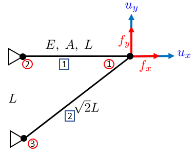
For our problem, we can see that we have four boundary conditions: u2x=u2y=u3x=u3y=0. The known nodal loads are f1y=−P. Furthermore we know the rod quantities E1=E2=E, A1=A2=A, L1=L and L2=2L.
We want to know the displacements in node 1, the reaction forces in nodes, 2 and 3 and all rod normal forces, stresses, strains and deformations.
The node 1 is said to be free, i.e., able to be translated in x and y. We say that node 1 has two degrees of freedom.
We now introduce the displacement field (vector) which corresponds to each degree of freedom.
u=⎣⎡u1xu1y⎦⎤
Additionally, we introduce the nodal load vector
f=⎣⎡f1xf1y⎦⎤
We will replace the known loads later, i.e., we will evaluate f1y=−P at a later time.
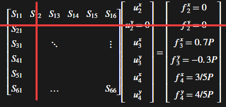
The problem is to find a relation between the loads f and the displacements u. This is done by computing the stiffness matrix for the structure such that
Su=f⇒u=S−1f
Equilibrium of an isolated node leads to the matrix AT directly, this approach is known as method of joints.
Setting up material relations leads to the Se matrix directly.
Thus having AT and Se gives
S=ATSeA⇒u=S−1f
Once the displacements are known, we can compute the rod quantities:
Step 3: Introduce the displacement vector and load vector
u=[u1xu1y]f=[f1xf1y]
Step 4: Rod fields
δ=⎣⎡δ1δ2δ3⎦⎤,N=⎣⎡N1N2N3⎦⎤
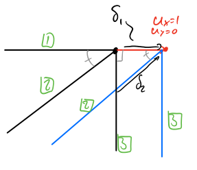
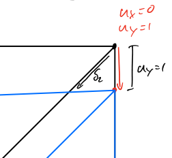
Step 5: Determine either AT by equilibrium using the method of joints or determine A using the unit displacements method. We shall do both and you can decide what method you prefer.
The boundary condition at node 1 means u1x=u1y=0 and at node two, we have the boundary condition u2y=0.
Determine the displacements, symbolically.
Set E=A=L=P=1 and plot the displaced structure.
Modify the boundary condition at node 2 to be u2y=−51EAPL and determine the rest of the displacements, plot!
Solution
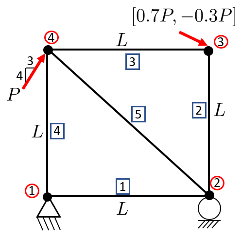
We start by posing equilibrium equations on nodes which are partly free, i.e., nodes 2, 3 and 4.
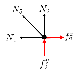
Node 2:
→:f2x=N1+1/2N5↑:f2y=−N2−1/2N5
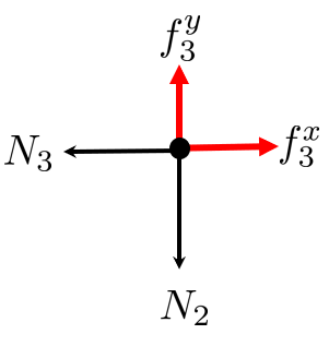
Node 3:
→:f3x=N3↑:f3y=N2
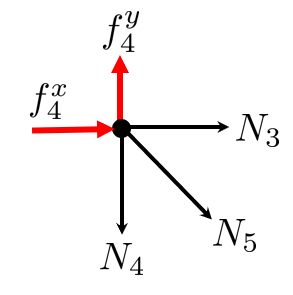
Node 4:
→:f4x=−N3−1/2N5↑:f4y=N4+1/2N5
Note how we are skipping node 1, since all degrees of freedom are prescribed to zero. We could add it though, and deal with eliminating equations later.
In order to visualize the displacements, we need numeric data, in this case, we were not provided with data, so we set everything to 1.
E = 1; A = 1; L = 1; P = 1;
u = double(subs(u))
u = 6x1
1.300007.77700.30007.07702.1000
We split the x and y components of the displacements into a matrix with the first column being the x-components and the second column being the y-components.
U = [00
u(1:2:end), u(2:2:end)]
U = 4x2
001.300007.77700.30007.07702.1000
Now, we shall create the topology of the structure, first the coordinates of our structure:
p = [00
L 0
L L
0 L];
Then the edge connectivity.
edges = [1223341424];
Now we can send this off to the patch function, which draws the whole structure in one simple line.
figure
patch('Faces',edges,'Vertices',p,'LineWidth',2)
axis equal
hold on
Now we shall overlay the undeformed structure with our deformed structure. We do this by adding the displacement field to our coordinate field such that
Pdeformed=Pundeformed+Us
where we need to scale the displacement field such that it shows the trend without being overly deformed.
In this case, the displacement u2y is not zero, and causes a reaction force which affects the whole structure. We deal with this by modifying the right hand side. In other words, we need to subtract the reaction forces which this displacement causes from the load vector. The reaction force is
We do this in Matlab by defining a variable for the prescribed degree of freedom.
presc = 2;
Then we modify the right-hand side
u = zeros(6,1);
u(presc) = -1/5*P*L/(E*A)
u = 6x1
0-0.20000000
fr = S(:,presc)*u(presc)
fr = 6x1
0.0707-0.270700.2000-0.07070.0707
f = f - fr
f = 6x1
-0.07070.27070.70000.10000.67070.7293
free = [1,3,4,5,6]; %Free degrees of freedom
S(free,free)
ans = 5x5
1.353600-0.35360.353601.00000-1.00000001.000000-0.3536-1.000001.3536-0.35360.353600-0.35361.3536
f(free)
ans = 5x1
-0.07070.70000.10000.67070.7293
Now we solve the for the free DOFs.
u(free) = S(free,free)\f(free)
u = 6x1
1.3000-0.20007.97700.10007.27702.1000
Now, let's visualize!
U = [00
u(1:2:end), u(2:2:end)]
U = 4x2
001.3000-0.20007.97700.10007.27702.1000
figure
patch('Faces',edges,'Vertices',p,'LineWidth',2)
axis equal
hold on
scale = 0.05;
patch('Faces',edges,'Vertices',p+U*scale,'LineWidth',1,'LineStyle',':')
plot(p(:,1),p(:,2),'ok','MarkerFaceColor','c','MarkerSize',14)
text(p(:,1)-0.01,p(:,2),cellstr(num2str([1:4]')))
fori=1:5
inod = edges(i,:);
xm = mean(p(inod,1));
ym = mean(p(inod,2));
text(xm,ym,num2str(i),'backgroundColor','y')
end
We can see a rather small displacement in the negative y-direction in node 2. Comparing the numerical values shows that all displacements are displaced slightly downward.