Applied Mechanics

Table of contents

Vector approach

Mechanics is all about modelling, meaning that we need to create mathematical models which describe the mechanics in order to solve for interesting entities. The physical problem is first simplified into a mechanical system, using assumptions. We need to keep track of all errors we introduce in such assumptions, this is where experience comes into play. And what we lack in experience we need make up with experimentation.

Preliminaries - vector properties

$\overrightarrow{\textrm{OA} }$ is defining the "origin vector" (ortsvektor), which is the vector going from the origin to the point A. We denote such vectors with an arrow.

A vector can also be denoted using bold lowercase letters, i.e., $\mathit{\mathbf{a} }$ or underlined $\underline a$ (easier to write on the board during a lecture).

The magnitude is computed using the Pythagorean theorem which is a special case of the Euclidean norm or 2-norm

where $a_x ,a_y$ and $a_z$ are the Euclidean components of the vector $\mathit{\mathbf{a} }$. A vector can also be disassembled into an unit vector and a magnitude:

$\mathit{\mathbf{a} }=a\;{\mathit{\mathbf{e} } }_a$, where ${\mathit{\mathbf{e} } }_a =\frac{\mathit{\mathbf{a} } }{|\mathit{\mathbf{a} }|}$

Let's start by defining some helper functions which we will use frequently.

First we clear the workspace, this is good practice in scripts, to avoid nasty bugs when using the same variables in the same document. For every problem, we begin by running the clear command in our script.

clear

Matlab is made for linear algebra and treats natively EVERYTHING as matrices, as such it sees no difference between a vector or a matrix. Matlab in fact is short for Matrix Laboratory.

In Matlab we can quickly compute the norm (magnitude) of a vector simply by using the function norm() which basically does $\sqrt{\mathbf{a} \cdot \mathbf{a} }$ .

Many times we need to compute the unit vector for some vector $\mathbf{a}$. Unfortunately there is no built in function in Matlab to do so. But we can create our own functions easily, the simplest way is to create an anonymous function.

normalize = @(a)a./norm(a);

Here, we use the built in function norm to compute the magnitude. The @(a) part defines the variable of the function. Let us try with $\mathbf{a} =\left\lbrack 3,4,0\right\rbrack$ since we expect the answer to be $\left\lbrack 3/5,4/5,0\right\rbrack$.

a = [3,4,0];
normalize(a)

ans = 1x3    
    0.6000    0.8000         0

As a test we take to norm of the result

norm(normalize(a))

ans = 1

OK!

Sometimes we need to compute the projection of vector $\mathbf{a}$ onto vector $\mathbf{b}$:

proj = @(a,b)dot(a,b)/dot(b,b)*b;

Let us test this by projecting $\mathbf{a}$ onto the $x$-axis, which is the same as taking the x-component of $\mathbf{a}$.

b = [1,0,0]

b = 1x3    
     1     0     0

proj(a,b)

ans = 1x3    
     3     0     0

OK!

Example 1.

Let us study the following problem

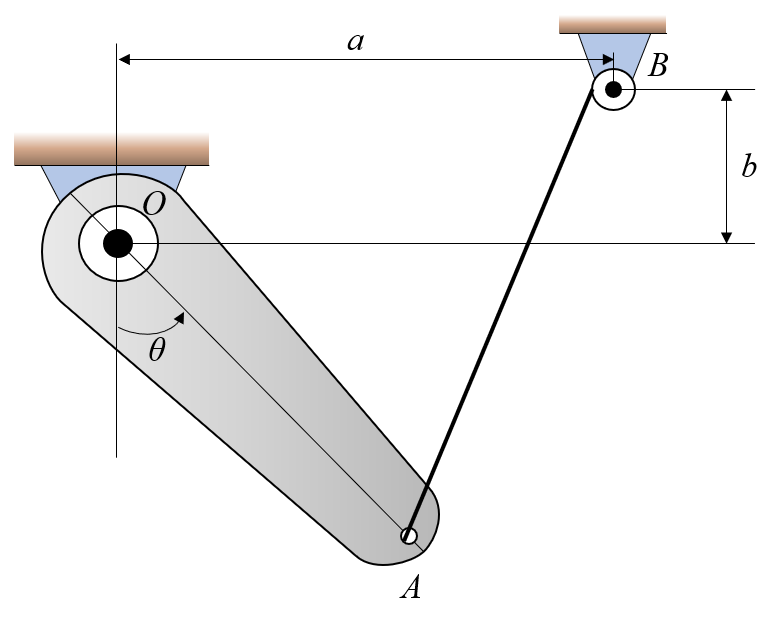
The arm OA can rotate freely around O and is actuated by the string attached in $A$ and around $B$. Let $a=400\mathrm{mm}$, $b=35\mathrm{mm}$ and $|\overrightarrow{\mathrm{OA} } |=350\mathrm{mm}$.

• Express the length $|\overrightarrow{\mathrm{AB} } |$ as a function of $\theta$ and find the minimum distance and at which $\theta$ this occurs for $\theta \in \left\lbrack 0,180\degree \right\rbrack$.

• How does the minimum distance vary with $b$?

Solution

Using the right-hand rule we define a coordinate system with $x$ positively to the right, $y$ positively up and thus $z$ is given positively outward from the screen.

Even if the problem is simplified into two dimensions (2D problem or plane problem), we will still use three dimensions in our computations, to ensure that the cross product function, cross(), works in Matlab.

The point $B$ is a fix point, it does not vary with $\theta$, so it is easiest to describe.

The point $A$ varies with $\theta$, using trigonometry we can identify a triangle and define the components. We begin with the unit vector.

Testing this is always a good idea, just set $\theta$ to some angles for which the outcome is trivial. For $\theta =0$ we expect to get ${\mathit{\mathbf{e} } }_{\mathrm{OA} } \left(\theta =0\degree \right)={\left\lbrack 0,\;-1,\;0\right\rbrack }^T$, which is the case, and for $\theta =90\degree$ we expect to get ${\mathit{\mathbf{e} } }_{\mathrm{OA} } \left(\theta =90\degree \right)={\left\lbrack 1,\;0,\;0\right\rbrack }^T$, which also is the case.

Now we can define

The vector $\overrightarrow{\mathrm{AB} }$ is given by taking the "head minus the tail"

And finally the magnitude of the length is given by

Now we will compute this in Matlab using symbolic expressions and plot the length as a function of theta to get a graphical solution, which is a perfectly valid solution to our problem.

clear
OB = [400, 35, 0].';
syms theta
eOA = [sind(theta), -cosd(theta), 0].';
OA = 350 * eOA;

AB = OB-OA

L = norm(AB)

figure
fplot(L,[0,180])
xlabel("\theta")
ylabel("L")
title("L(\theta)")

You can now zoom in on the minimum point to get the answer (to an arbitrary precision), $L$ has its lowest value of $51\mathrm{mm}$ at $\theta =95\degree$.

We could of course compute the derivative, set it to zero and solve for theta to get the minimum value.

dL = diff(L,theta)

theta1 = solve(dL==0,theta)

We have a problem, we are getting weird results, in fact we expect to get infinitely many results since the solution is cyclic.

We can switch to a numerical solver to find the answer

theta1 = vpasolve(dL==0, theta, 95)

Here vpasolve(), uses a variant of the Newton-Raphson root finding method to find the root using an initial value.

Let us vary $b\in [-10,50]$.

figure; hold on
for b = [-10,0,10,20,30,40,50]
    OB = [400, b, 0].';
    AB = OB-OA;
    L = norm(AB);
    fplot(L,[0,180], 'Displayname', ['b: ',num2str(b)])
end
legend show
xlabel("\theta")
ylabel("L")
title("L(\theta)")

Visualization gives an additional dimension to the understanding.

If in doubt, write some visualization code!

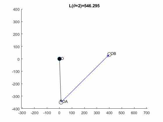
theta = 0;
eOA = [sind(theta), -cosd(theta), 0].';
OA = 350 * eOA;
AB = OB-OA;
L = norm(AB);

figure; hold on;
axis([-50,450,-400,400])
plot(0,0,'o','MarkerFaceColor','k','MarkerSize',10)
text(10,5,'O')

plot(OA(1),OA(2),'ok','MarkerFaceColor','w','MarkerSize',10)
text(OA(1)+10,OA(2)+10,'OA')

plot(OB(1),OB(2),'ok','MarkerFaceColor','w','MarkerSize',10)
text(OB(1)+10,OB(2)+10,'OB')

quiver(0,0,OA(1),OA(2),0,'k')

quiver(OA(1),OA(2),AB(1),AB(2),0,'b')

Interactive example