Table of contents
We start with kinematics and the mathematical descriptions of a bodies position, velocity and acceleration. This is the foundation of dynamics, including kinetics.
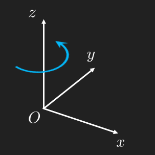
Assume an universal coordinate system and stick to it! We can choose between cartesian, normal and polar coordinate systems.
If a body has an insignificant rotation compared to the path its center of gravity travels, it is said to be a particle. In later chapters we will make an proper introduction to generalized Newtonian-Euler motion equations, but for now, suffice to say if either the rotational acceleration or the size of the body is small enough, then we can neglect the change of angular momentum
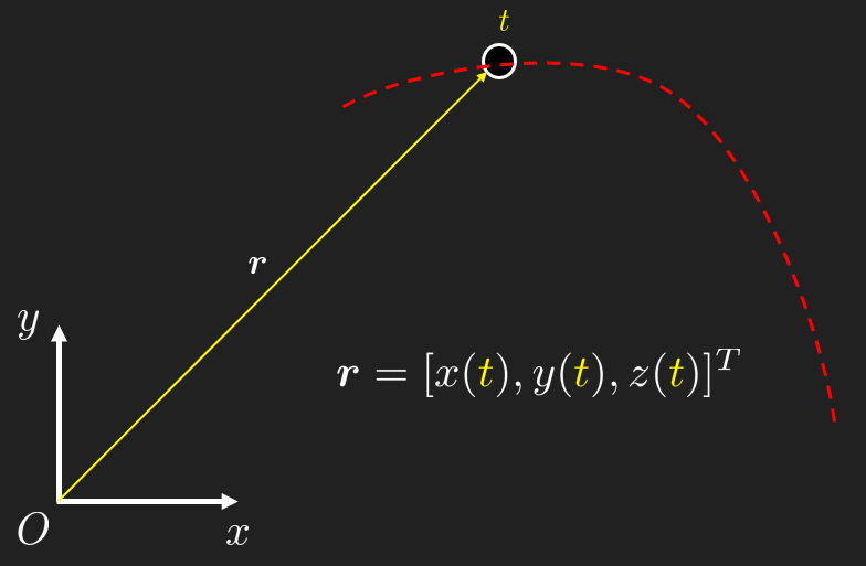
The position of a bodies center of gravity as a function of time can be expressed using the position vector where each component is a function of the same independent variable . The components are called coordinate functions and is known as the parameter curve with the parameter . The parameter curve is also known as the curve or path.
The mean velocity between two positions and can be described as . In the limit where we get the time derivate of the position vector, known as the velocity vector
As can be seen in the animation, the velocity vector at is always tangential to the path.
The dot notation in or in (a.k.a. Newton's abomination) comes from Newton who studied dynamic problems and needed to develop the mathematics to deal with these problems. The mathematics came to be known as calculus which was expanded and is really made up by a great many contributors (Leibnitz, Lagrange). see e.g., this video for an historical overview.
The magnitude of the velocity vector, , is known as the speed. The difference between velocity and speed being that velocity also contains information about the direction of the object.
Similarly, the acceleration is given by the change of velocity over time, . The average acceleration at time can be formulated as
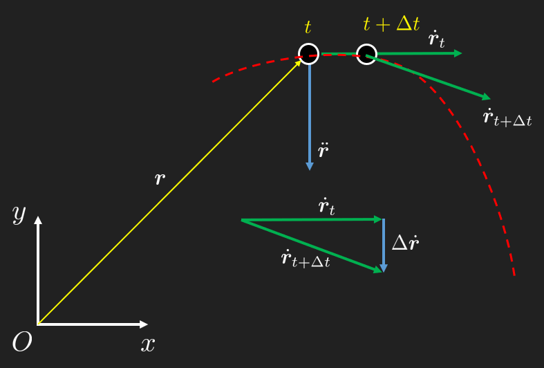
From the animation we can see that the acceleration is pointing inwards, towards the center of curvature. Also, we see that the acceleration in general differs from the direction of the position vector. The acceleration is in fact orthogonal to the velocity as we shall see in the following sections.
In the following sections, we will analyze curvilinear motion in more detail, but next we'll discuss the special case of no curvature...
In the special case of rectilinear motion (motion without curvature), such as described in the figure below
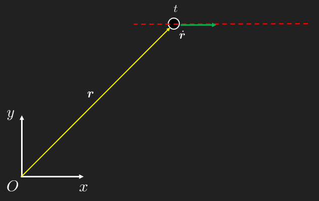
we sometimes use the (simple) scalar notation
We can express these scalar values using the Leibniz notation for time derivative
solving for the time increment , we get
from which we get
Which is convenient to use in special cases where we are not interested in time explicitly, but should be used with care and really be avoided all together, instead the proposed working method is described in what follows.
Working purely with the scalar notation from the previous section is troublesome. A strong recommendation is to avoid the use of derived formulas often found in classical books in mechanics and formularies, since it is often more tedious to figure out the assumptions under which these formulas are valid than to create a model using the differential equations directly. Many ready-to-go formulas assume the acceleration to be constant. We shall also refrain from using the notations for varying position, velocity and acceleration since it is harder to let go of the "thinking by formularies" and move towards "Concept Based Modeling" with "Computational Thinking". Instead use along with knowledge of differential equations!
Remember that the derivative and integral operator works naturally on vectors i.e., and .
The acceleration (vector) is the time derivative of the velocity (vector) , or the second time derivative of the position (vector).
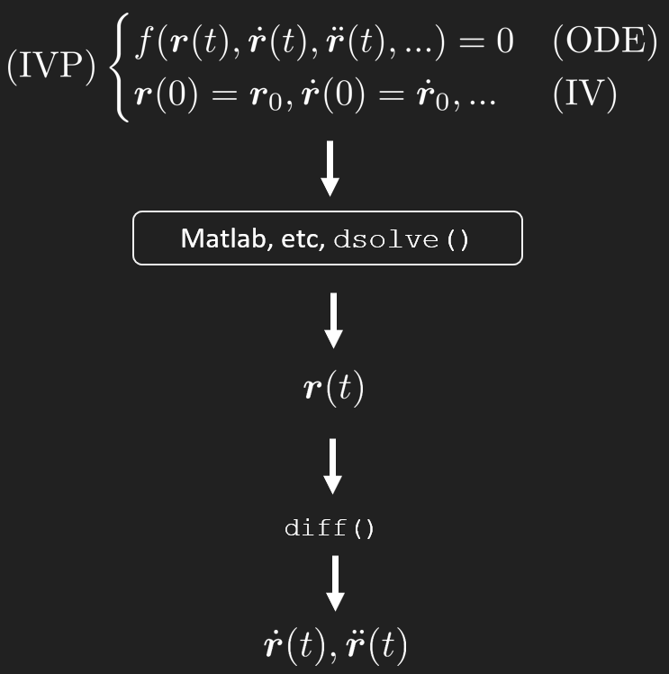
In what follows we shall rely more on working with the vector form of and formulate the differentials as ordinary differential equations which we can easy solve using either a symbolic differential equation solve, e.g., dsolve() or numerically by utilizing e.g., the Euler method.
The modern workflow in computational dynamics can be summarized in the figure below
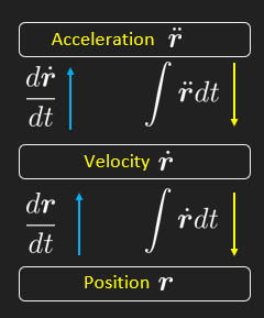
To get between the different quantities position, , velocity and acceleration we take the derivative in one direction and integrate in the other. In practice one does not typically manually integrate expressions, one typically solves an ordinary differential equation (ODE) instead, which takes us all the way down to which is the solution to an ODE. Then we can take the derivative to determine the needed quantities. This is typical for a symbolic solution. Non-linear ODEs, on the other hand, are typically solved using various numerical algorithms which will first generate velocity, on the way down to the final position .
Newtonian physics is formulated as the kinetic equation
which is a second order ODE, but in kinematics we se equally often differential equations of first order. Regardless, it is very convenient to solve any equation using matlab.
We formulate an ODE which needs to be (at least piece-wise) valid for all and apply initial conditions at the beginning of the analysis and/or at some other known state as boundary conditions (BC) to fix the unknown constants, where the number of constants depend on the order of the differential equation.
In this approach, the time is the central parameter that ties the quantities (, and ) together, which is why it often pops out in the solution without being maybe being explicitly asked for. This is the nature of Newtonian mechanics, it is inherently transient, meaning the state of the body is known for every time step. As we shall see in upcoming chapters, there are other methods which can greatly simplify calculations and modeling if the dependency of time is not important, e.g., equation (7). Note however that a complete dynamic analysis requires the solution of the ODE.
The inquiries to the model can be essentially divided into two categories:
Explicit time dependent, the equations are explicitly functions of a time variable, e.g., , such that we can evaluate the quantities for a given time.
Implicit time dependent, where we want to know a quantity expressed as a function of another quantity and thus we need to solve an equation to get the time which is common for both quantities. E.g., find the velocity when the position is a given value, .
There are several types of bases (or coordinate systems) on which we can formulate kinematic expressions and work with derivatives, traditionally this is done to simplify calculations, done by hand, and the resulting symbolic expressions.
We shall here derive the most common coordinate systems and their base vectors such that this projection can be done.
Cartesian, our typical -system, here denoted, , with , and .
Polar or circular (2D) or cylindrical (3D), .
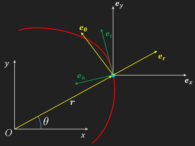
Natural (tangent, normal and bi-normal), .
Sometimes the bases can be denoted simply , and , but throughout this treatment we will try to be explicit and denote en basis vectors and unit vectors with a specific sub-index for clarity.
The tangent vector is always pointing in the parameter direction, tangential to the path and is defined as the direction of the velocity
The normal vector is perpendicular to and always points inwards to the center of curvature
here, suddenly a time derivate of a unit vector appears, see this section for an explanation.
Finally the lesser known bi-normal vector is defined as the cross product between the tangent and normal vectors,
which defines a right-hand system.
Note that for planar problems (2D) .
has the same direction as and is given by
is given by
In order to ensure orthogonality of two vectors, we can take their dot product, if the resulting scalar is zero, they must be orthogonal. If two vectors are parallel then their dot product must be one, i.e., . Now we can take the time derivative of this expression
Also note that typically .
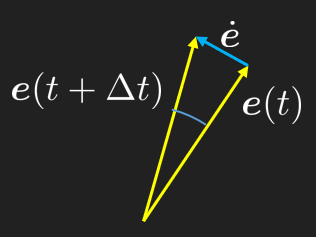
So at the limit we clearly see that .
Let
normalize = @(v)v/sqrt(v(:).'*v(:));
syms t positive
syms theta(t)
r = [cos(theta(t)),sin(theta(t))].'We compute the normalized vector
e_r = simplify(normalize(r))The time derivative of is then given by
e_r_dot = simplify(diff(e_r,t))What we computed above is a scaled direction which is perpendicular to the direction vector . Note that the time derivative of pops out from the chain rule, which is why necessarily since necessarily. Note that the direction of rotation is given by the sign of i.e., {-1,1}.
The above we re-write in Newton notation and define the basis vector as
Thus we can get the perpendicular vector, , by normalizing , i.e.,
e_theta = subs(simplify(normalize(e_r_dot)), diff(theta,t), 'theta_dot')Here we can see that only returns the sign of . Thus in this example and we get
Thus we have shown that
We shall here derive the kinematic equations explicitly in polar coordinates. Note again that in practice, working with a symbolic math manipulator like matlab, we can just formulate and and project onto the base. There is no need to learn the derived expressions below by heart in a modern workflow, instead we explore the connections between these entities and their physical meaning.
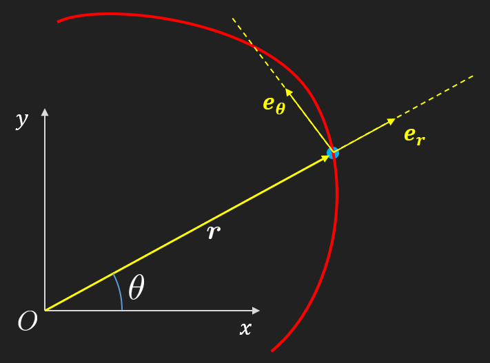
We begin by stating the earlier established bases.
We can express the position vector using the distance and base
where is the scalar length of the position vector.
Taking the derivative of the position vector we get, using the product rule
and with from (17) we have
where
is recognized as the angular velocity.
Taking the time derivative of the expression for velocity above we get
and with and we have the expression of the acceleration vector expressed in polar coordinates
Arguably more important are the kinematic relation expressed in Natural coordinates and even more useful are the acceleration terms which are split into normal and tangential directions. Here we shall derive these expressions explicitly, but note that we can always get these by just projecting the total velocity or acceleration vector onto any bases. Thus, there is no need to know these formulas or use them only for the sake of computing the quantities in one of these special bases.
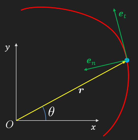
We begin by stating the earlier established bases.
Next, we introduce the center of curvature, , at some point and the corresponding curvature radius . We then can fit a circle arc length in the neighborhood of such that we get a constant radius for an infinitesimal circle arc angle . This way we can get a relation between the section distance and the angle
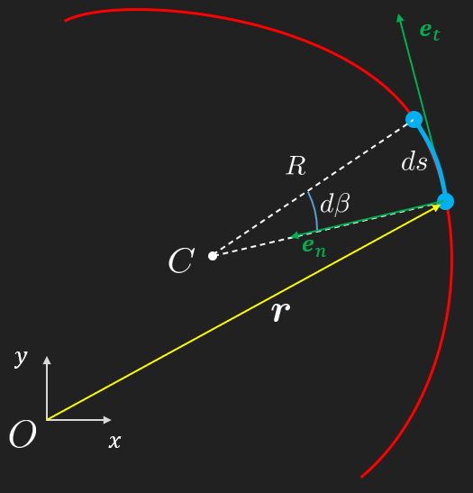
This circle arc length relation, along with the Pythagorean theorem and trigonometry is a corner stone in dynamics and the main building blocks in our modelling toolbox.
We remember the definition of velocity as and using the arc length relation we get
This relation is useful for when the angular rate is sought.
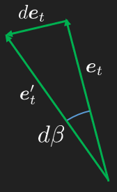
For a small change by we get the perpendicular direction which has the same direction as , we can thus formulate the relation
Thus we arrive at the relation
Since we get
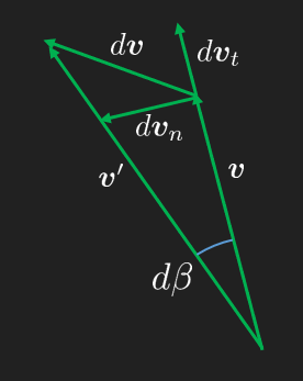
and with (36) we get
From this expression we note that we always have an acceleration as long as there is non-zero velocity and a curved path.
This split into the normal and tangential directions will be revisited and used once we get to the kinetics chapter.
The theory on curves is extensive and belongs to the field of mathematics called differential geometry. Here we shall only introduce som very basic concepts, such as the curve length, for which there might not exist a closed form solution, it needs to be integrated over all small contributions such as
This can be useful if the derivatives are needed to be expressed as instead of which can lead to simpler expressions, but since is a function of it does not make the practical computations easier when working computer based.
Another important concept is the curvature , which as we can see tends to zero as the curvature radius tends to infinity, which makes sense for a flat path. The curvature center is given by
This center-point lies in the center of what is known as the osculating circle, named by Leibniz (Circulus Osculans), it is the best fitting circle to the curve at the time . We note that the Natural coordinates are mostly used for this type of analysis.
The torsion of a curve, is a measure of how much a curve is being bent into the third dimension (compared to the curvature). Think of it like the pitch of a screw. Both the expressions for curvature and torsion are tedious to derive, hence we just state them here
where denotes the third order derivative of time, also known as jerk or jolt, for higher order time derivatives see this list.
Let us work out the curvature and torsion on a simple example, let
clear
syms R t positive
r = R*[cos(t), sin(t), 0].'r_dot = @(r) diff(r,t);
r_ddot = @(r) diff(r,t,2);
r_dddot = @(r) diff(r,t,3);
kappa = @(r) simplify( norm(cross(r_dot(r),r_ddot(r))) / norm(r_dot(r))^3 );
tau = @(r) - dot(cross(r_dot(r),r_ddot(r)), r_dddot(r)) / norm( cross(r_dot(r),r_ddot(r)) )^2;
kappa(r)tau(r)The results seem reasonable, torsion is zero since the path is zero in the -direction.
Finally we visualize the osculating circle on its journey accompanying a particle moving along the path
clear
syms t positive
y = 1*sin(2*t)*t^0.5;
y = matlabFunction(y);

r = [t,sym(y),0]r_dot = diff(r,t);
r_ddot = diff(r,t,2);
e_t = matlabFunction( simplify(r_dot/norm(r_dot)) );
e_n = matlabFunction( diff(e_t, t)/norm(diff(e_t, t)) );
e_t_dot = diff(r_dot/norm(r_dot),t);
e_t_dot_norm = matlabFunction(simplify(norm(e_t_dot)) );
r_dot = matlabFunction(r_dot);
r_ddot = matlabFunction(r_ddot);
figure
fplot(y,[0,10], 'Linewidth',2)
axis equal
xlabel('$x$','Interpreter','latex')
ylabel('$y$','Interpreter','latex')
c_bg = [33,33,33]/255;
set(gcf,'Color',c_bg)
set(gca,'FontSize',14,'FontName','Times','Color',c_bg,'XColor','w','YColor','w','ZColor','w')
hold on
box off
t = 1.2;
x = t;
e_t_N = e_t(t);
e_n_N = e_n(t);
c_green = [0, 176, 80]/255;
c_blue = [0,176,240]/255;
v = r_dot(t)v = 1x3
1.0000 -1.3072 0kappa = norm(cross(r_dot(t),r_ddot(t))) / norm(r_dot(t))^3kappa = 0.9946R = double( norm(v)/e_t_dot_norm(t) )R = 1.0054R = 1/kappaR = 1.0054r_N = [t, y(t),0];
r_C_N = r_N + e_n_N*R;
hc = plot(r_C_N(1), r_C_N(2),'ro','MarkerFaceColor','r','MarkerSize',3);
tt = linspace(0,2*pi,100)';
circle = @(R,r)R*[cos(tt),sin(tt)]+[r(1), r(2)]circle =
@(R,r)R*[cos(tt),sin(tt)]+[r(1),r(2)]C = circle(R,r_C_N);
hcircle = plot(C(:,1), C(:,2),'r-');
hp = plot(x,y(t),'ko','MarkerFaceColor','k','MarkerSize',8);
het = quiver(x,y(t), e_t_N(1), e_t_N(2), 1, 'Color',c_green, 'Linewidth',2);
hen = quiver(x,y(t), e_n_N(1), e_n_N(2), 1, 'Color',c_blue, 'Linewidth',2);
axis([0,10,-3,3])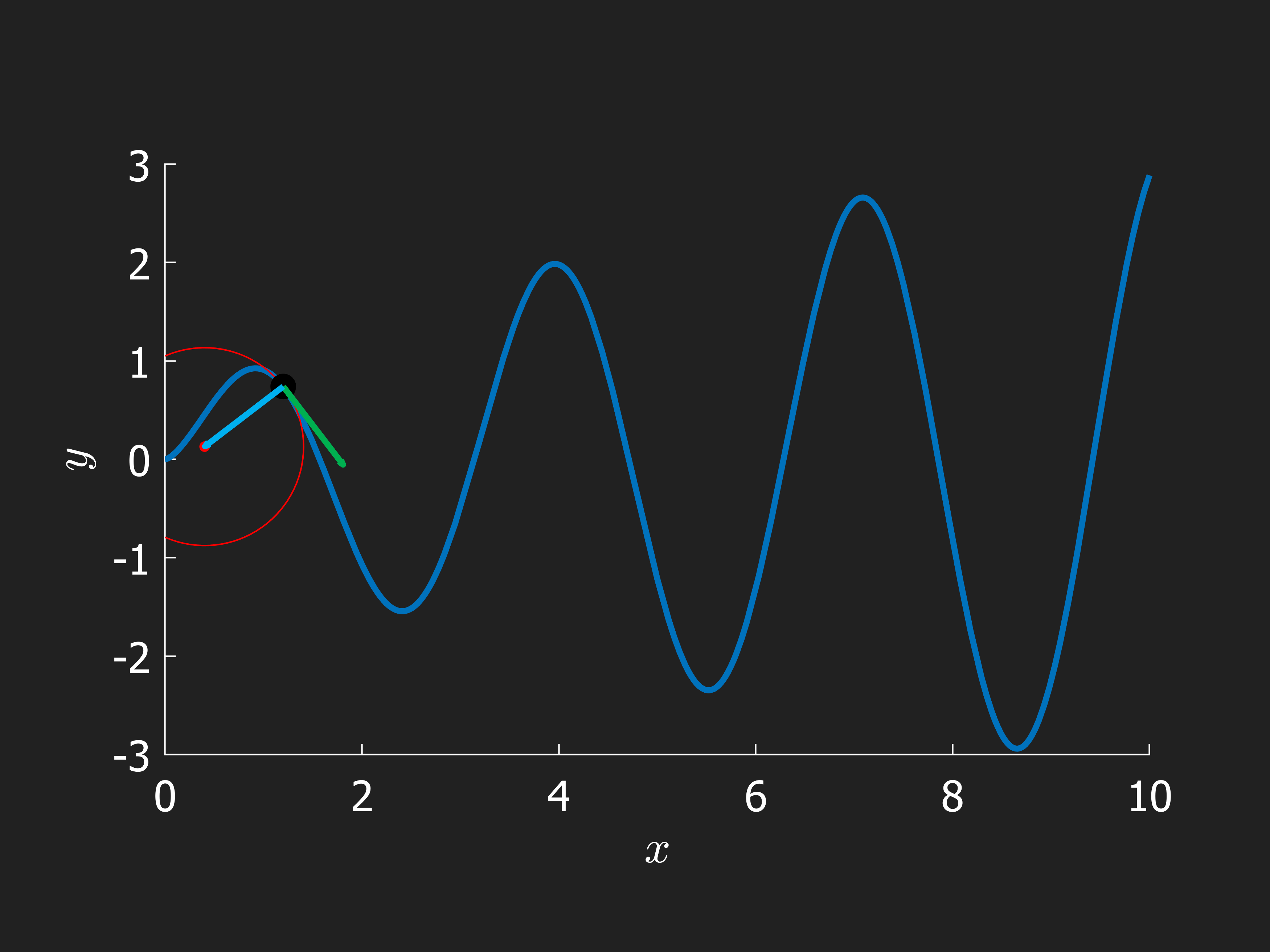
%
% for t = linspace(0,10,20)
%     x = t;
%     e_t_N = e_t(t);
%     e_n_N = e_n(t);
%     kappa = norm(cross(r_dot(t),r_ddot(t))) / norm(r_dot(t))^3;
%     R = 1/kappa;
%     r_N = [t, y(t),0];
%     r_C_N = r_N + e_n_N*R;
%     C = circle(R,r_C_N);
%     set(hp, 'XData', x, 'Ydata', y(t))
%     set(het,'XData', x, 'Ydata', y(t),'UData',e_t_N(1),'VData',e_t_N(2))
%     set(hen,'XData', x, 'Ydata', y(t),'UData',e_n_N(1),'VData',e_n_N(2))
%     set(hc, 'XData', r_C_N(1), 'Ydata', r_C_N(2))
%     set(hcircle, 'XData', C(:,1), 'Ydata', C(:,2))
%     axis([0,10,-3,3])
%     drawnow
% endA special case of curvilinear motion is planar circular motion.
Let us study the case of a particle in polar coordinates using the arm below
We begin by expressing the particles position
clear

syms theta(t) r(t)

rr = r*[cos(theta), sin(theta)].'Then we let matlab compute the derivatives
rr_dot = diff(rr,t);
syms r_dot theta_dot r_ddot theta_ddot
rr_dot = subs(rr_dot, [diff(r,t), diff(theta,t)], [r_dot,theta_dot])rr_ddot = diff(rr,t,2);
rr_ddot = subs(rr_ddot, [diff(r,t,2), diff(theta,t,2)], ...
[r_ddot, theta_ddot]);
rr_ddot = subs(rr_ddot, [diff(r,t), diff(theta,t)], ...
[r_dot, theta_dot])In the above expressions, we made the derivatives easier to read by converting to Newtonian notation. Clearly, Matlab can handle tedious derivation.
Now, we define the polar bases
e_r = [cos(theta), sin(theta)].';
e_theta = [-sin(theta), cos(theta)].';
where is orthogonal according to the right-hand rule (rotate 90 degrees counter clockwise).
Now just project the Cartesian vectors onto the polar bases. We can get away with the "low budget" projection since the bases have unit length, i.e., . We recall that the dot product is just a matrix multiplication
r_dot_rtheta = simplify([rr_dot.'*e_r, rr_dot.'*e_theta])r_ddot_rtheta = simplify([rr_ddot.'*e_r, rr_ddot.'*e_theta])We can see that we end up with the same expressions as we have tediously derived using the classical approach in the section on polar coordinates above.
For the special case of circular motion, we set the derivatives of to zero
r_dot = 0; r_ddot = 0;
v = subs(r_dot_rtheta)a = subs(r_ddot_rtheta)To summarize planar circular motion: with a constant , we have and since . Note especially the centripetal acceleration , it is directed in the negative direction of , towards the center of the circle.
If the rotational velocity is constant, i.e., if or then we only have centripetal acceleration, caused by a curvilinear motion and perpendicular to the tangent direction, directed inwards, towards the center.
Note that we can express bases using the cross product
which is very convenient since circular motion is common and we often have angular velocity as input data, thus we can formulate
Another easy way is to explicitly rotate the base by 90 degrees into the direction of curvature, the drawback is we need to know which direction to rotate into, which is why the previous method is preferred, since the direction of rotation is determined by the sign of the angular velocity .
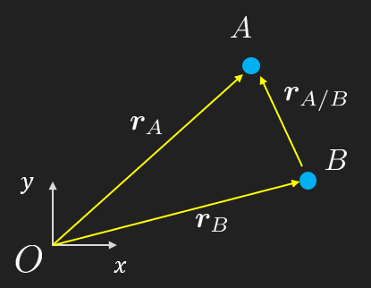
Many times we can express position and motion (velocities and acceleration) relative to some other point rather than the origin. This is done such that the modeling becomes significantly easier and less error prone. Besides, in real world applications, engineers need to make measurements and many times it is more accurate to make relative measurements rather than absolute. This approach is called relative motion analysis and will be used extensively in rigid body dynamics.
If we know the position of particle as well as the relative position of particle with respect to , that is (Can be read: A seen from B) we can express the absolute position of as
Again it might be more convenient to express and than directly.
If the position vectors are expressed as variables of time, we can differentiate them with respect to time and get
and
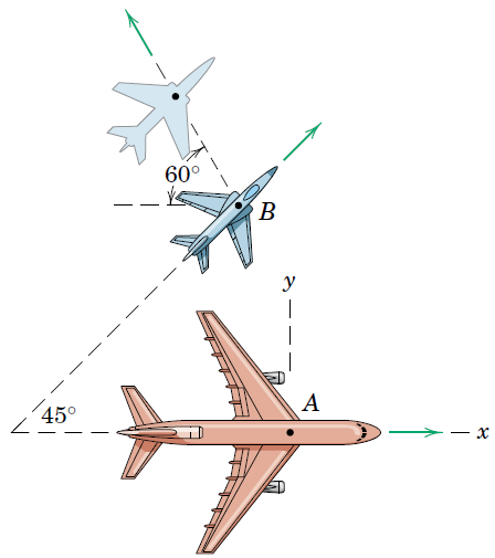
Passengers in the A380 flying east at a speed of 800 km/h observe a stunning JAS 39 Gripen passing underneath with a heading of in the north-east direction, although to the passengers it appears that the JAS is moving away at an angle of as shown in the figure. determine the true velocity of the JAS 39 Gripen.
Solution:
clear
syms v_B v_BA

v_A = 800
v_A = 800V_A = v_A*[1;0]V_A = 2x1
800
0e_B = [cosd(45); sind(45)]e_B = 2x1
0.7071
0.7071V_B = v_B*e_Be_BA = [-cosd(60); sind(60)]e_BA = 2x1
-0.5000
0.8660V_BA = v_BA*e_BANow we can formulate the equation, which is good to write out, that way we can see the number of variables and the number of equations.
eqn = V_B == V_A + V_BAWe then solve for the unknowns and convert to numerical values.
[v_B, v_BA] = solve(eqn,[v_B,v_BA])v_B = vpa(v_B,5)v_BA = vpa(v_BA,5)To conclude, the JAS is moving away from the passengers at 585 km/h and its absolute speed is 717 km/h.
The acceleration performance of a new solar car is being tested at the Jönköping airfield. The JTH students are measuring time against velocity and the data is presented as two vectors. Create a suitable continuous function of the speed and determine how far the car has traveled at the last measurement point. Plot the distance - time curve as well as the acceleration curve.
Given data:
T =  [1.1486
      2.0569
      3.1485
      4.0443
      5.0165
      6.2552
      7.1682
      8.2789
      9.209
      10.175];
V = [9.1023
     16.245
     22.732
     26.446
     33.052
     36.889
     41.304
     43.496
     45.861
     48.319];
Solution:
Fit a quadratic function to the data, in general we have:
where in our case. On matrix form this becomes:
Solve for the constants, , using the least squares method:
syms t
n = 2;
t.^[0:n]X = @(t)t.^[0:n];X = X(T)X = 10x3
1.0000 1.1486 1.3193
1.0000 2.0569 4.2308
1.0000 3.1485 9.9131
1.0000 4.0443 16.3564
1.0000 5.0165 25.1653
1.0000 6.2552 39.1275
1.0000 7.1682 51.3831
1.0000 8.2789 68.5402
1.0000 9.2090 84.8057
1.0000 10.1750 103.5306c = (X'*X)\X'*Vc = 3x1
1.0555
7.7545
-0.3097c = X\Vc = 3x1
1.0555
7.7545
-0.3097The constants can now be multiplied with
t.^[0:n]to get the velocity, here using 4 significant numbers
v = vpa(t.^[0:n]*c,4)Let us plot the data and the quadratic function
figure; hold on
plot(T,V,'ro')
fplot(v,[0,max(T)],'b-')
xlabel('Time, t [s]')
ylabel('Velocity, v [m/s]')
grid on
tn = linspace(0,max(T),100);
vn = double(subs(v,t,tn));
area(tn, vn, 'FaceColor','b','FaceAlpha', 0.2)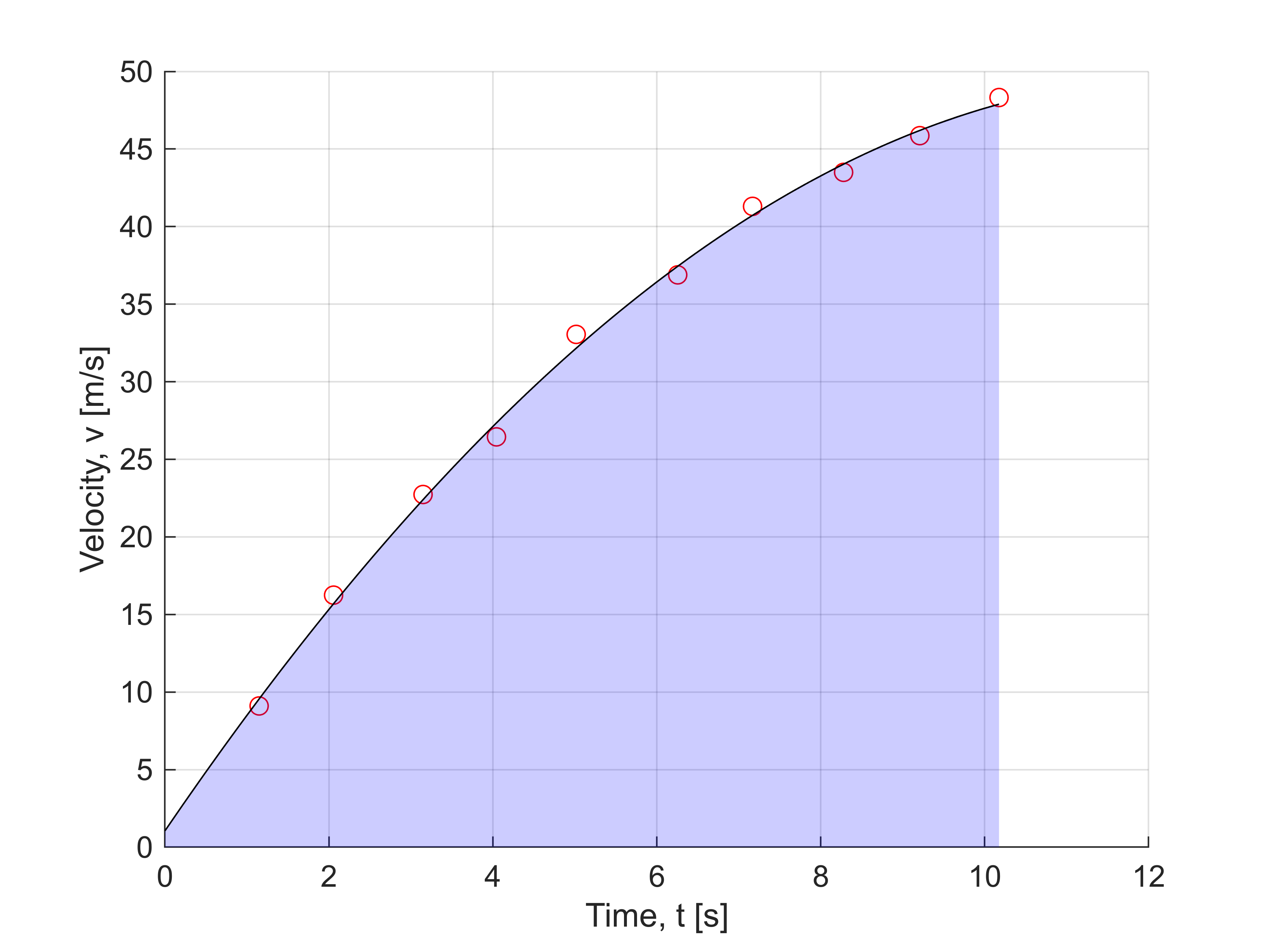
The fit looks quite good, let us look at other methods of applying the least squares method. In Matlab the \ operator is really only short for linsolve(), which is a powerful function, and for matrix system which are not square, linsolve() automatically computes the least squares solution. Let's try it out
X\Vans = 3x1
1.0555
7.7545
-0.3097In addition to this, there are specific functions for fitting polynomials to data, called polyfit():
[c, S] = polyfit(T,V,2)c = 1x3
-0.3097 7.7545 1.0555
S =
R: [3x3 double]
df: 7
normr: 1.8563Now back to the problem at hand, first the acceleration, we just integrate the velocity
a = vpa(diff(v,t),4)Next we plot the acceleration
figure;
fplot(a,[0,max(T)],'m-')
xlabel('Time, t [s]')
ylabel('Acceleration, a [m/s^2]')
grid on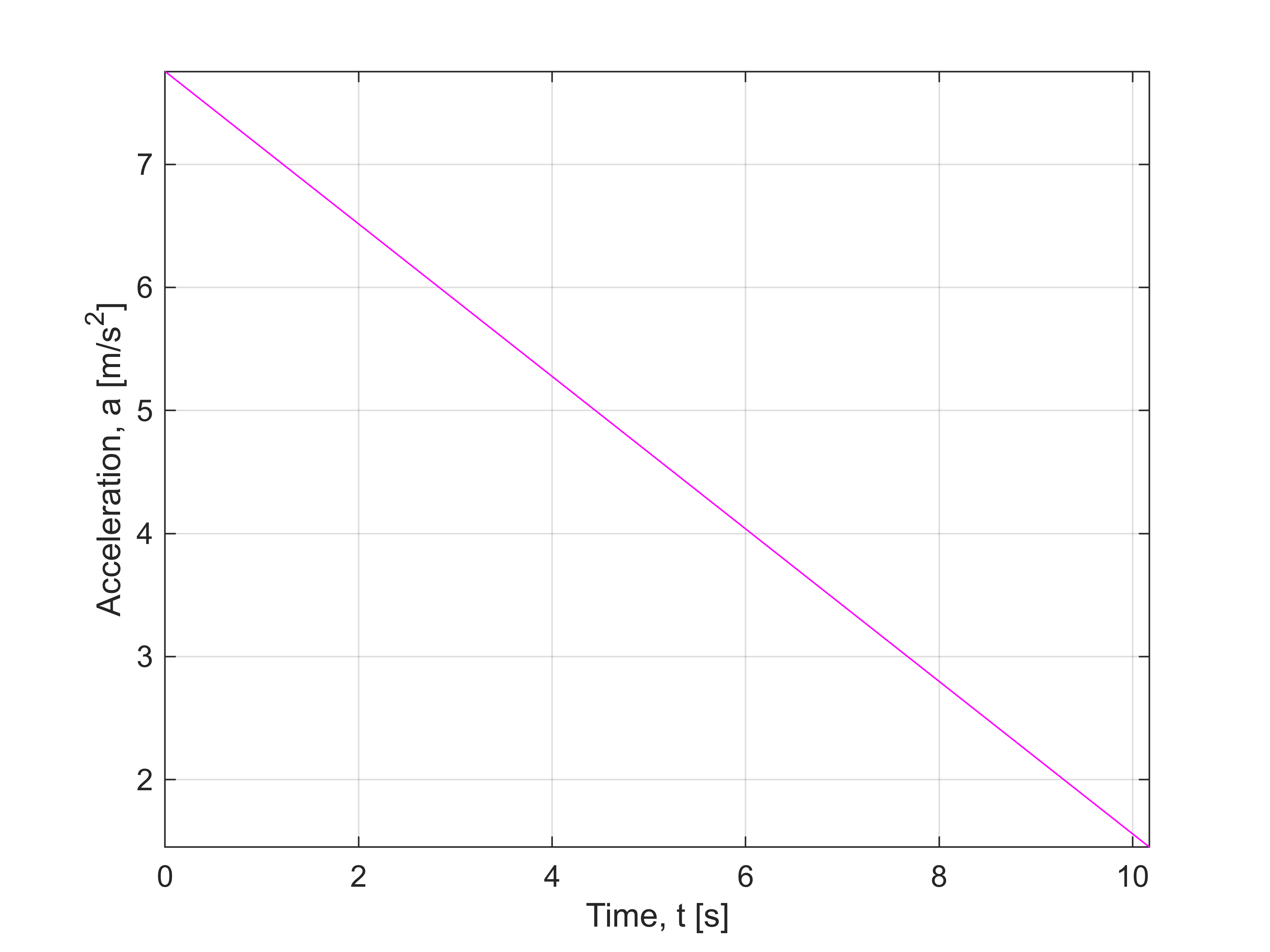
We note that the car is linearly de-accelerating.
Finally, the total distance, which is given by integrating the velocity over the complete time range, i.e., we compute the area under the velocity curve
s = int(v,[0,max(T)])The total distance traveled at the last data-point is 303m.
A particle moves along the -axis with an initial velocity at the origin when . For the first 4 seconds it has no acceleration, and thereafter it is acted on by a retarding force which gives it a constant acceleration . Compute the velocity and the -coordinate of the particle for the conditions of s and s and find the maximum positive -coordinate reached by the particle.
Solution:
Here we have written the given data as an ODE with initial conditions, now we can solve
clear
syms x(t)
DE = diff(x,t,2) == -10v = diff(x,t)IV = [v(4) == 50, x(4) == 50*4]We first solve the ODE to get the position, which we then can differentiate w.r.t. time and answer the inquiries
x(t) = dsolve(DE,IV)v(t) = diff(x,t)v(8)v(12)t_max = solve(v==0, t)x(t_max)v(t) = piecewise(0 <= t < 4, 50, ...
4 < t, v)Finally a graph over the situation
figure
hold on
fplot(50*t, [0,4], 'b', 'Linewidth',2)
fplot(x, [4,12],'r', 'Linewidth',2)
xlabel('Time $t$ [s]','Interpreter','Latex')
ylabel('Distance $s(t)$ [m]','Interpreter','Latex')
The area under the graph
tn1 = linspace(0,4,100);
tn2 = linspace(4,12,100);
xn = matlabFunction(x);
area(tn1, 50*tn1, 'Facecolor','b','FaceAlpha',0.2)
area(tn2, xn(tn2), 'Facecolor','r','FaceAlpha',0.2)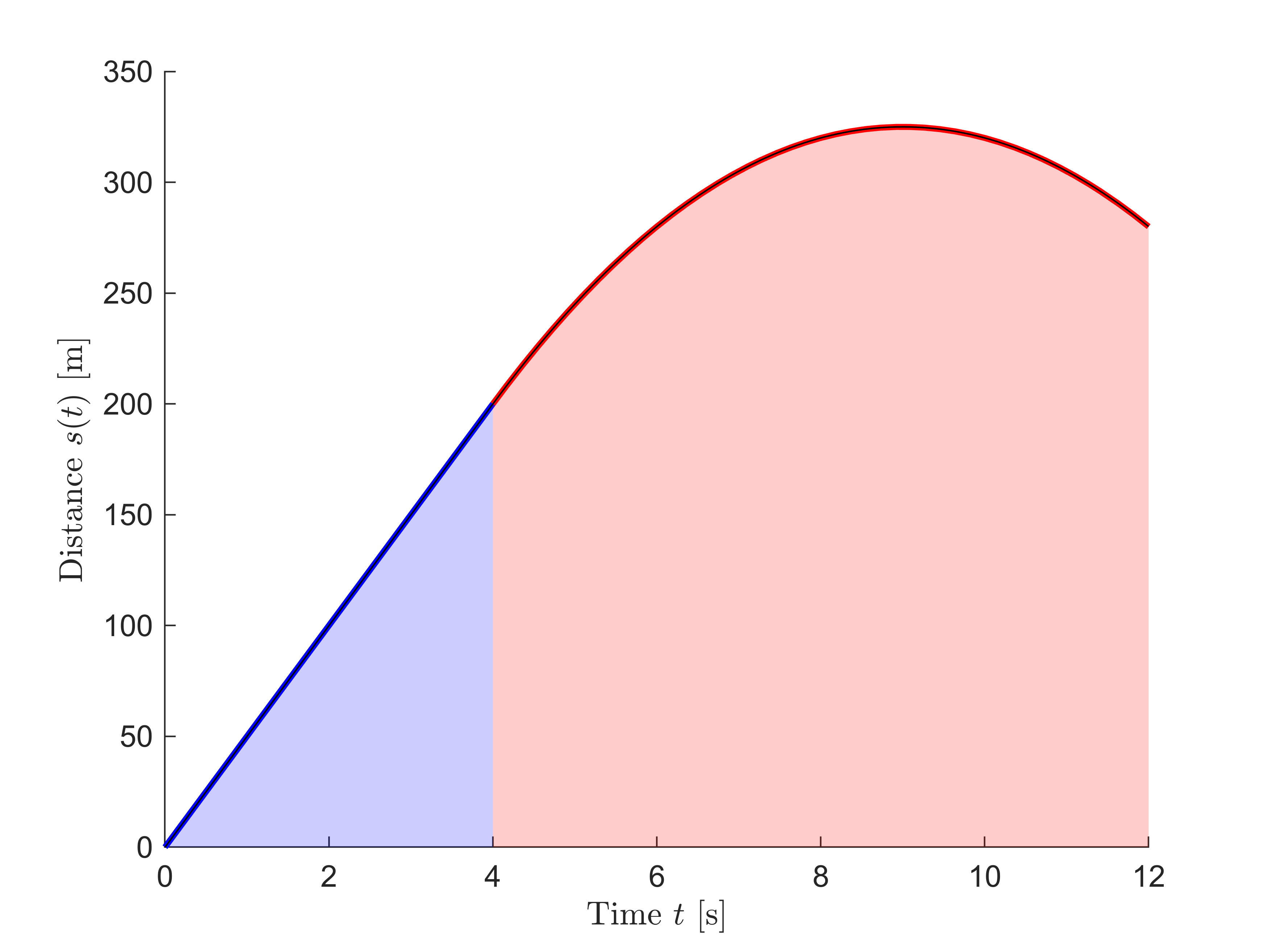
And the velocity graph
figure; hold on
fplot(v, [0,12], 'b', 'Linewidth',2)
xlabel('Time $t$ [s]','Interpreter','Latex')
ylabel('Velocity $v(t)$ [m/s]','Interpreter','Latex')
axis([0,12,-30,55])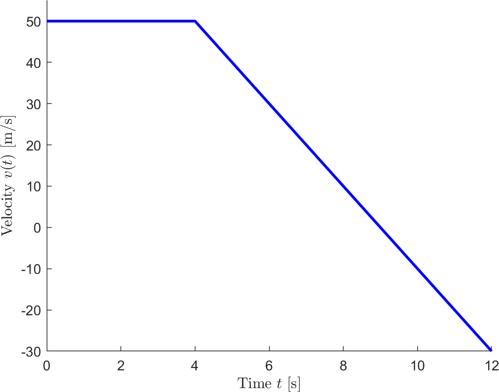
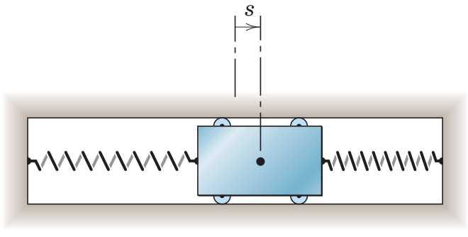
A spring mounted slider is being moved along the -axis and has an initial velocity m/s in the s-direction as it crosses the mid-position where and . The two springs together exert a retarding force to the motion of the slider, which gives it an acceleration proportional to the displacement but oppositely directed and equal to , where . Determine the displacement, velocity and acceleration of the slider and plot.
syms x(t) k

syms v0
DE = diff(x,t,2) == -k^2*xv = diff(x,t)BV = [v(0) == v0, x(0) == 0]x(t) = dsolve([DE,BV])x = simplify(x)v = diff(x,t)a = diff(v,t)x = subs(x,[v0, k],[2,4])v = subs(v,[v0, k],[2,4])a = subs(a,[v0, k],[2,4])t1 = 2*pi;
figure; hold on;
fplot(x,[0,t1],'Linewidth',2,'DisplayName','Position [m]')
fplot(v,[0,t1],'Linewidth',2,'DisplayName','Velocity [m/s]')
fplot(a,[0,t1],'Linewidth',2,'DisplayName','Acceleration [m/s^2]')
set(gca,'XAxisLocation','origin')
legend('Show')
xlabel('Time $t$ [s]','Interpreter','Latex')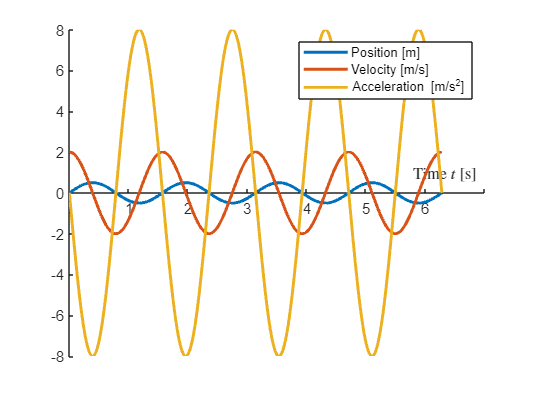
tn = linspace(0,t1,100);
vn = matlabFunction(v);
figure; hold on
fplot(v, [0,t1], 'Linewidth',2,'DisplayName','Velocity [m/s]')
area(tn, vn(tn), 'FaceColor','b','FaceAlpha',0.2,'DisplayName','Position [m]')
set(gca,'XAxisLocation','origin')
legend('Show')
xlabel('Time $t$ [s]','Interpreter','Latex')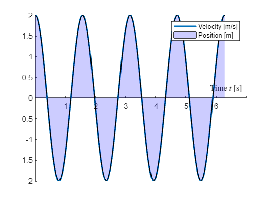
The total area is the distance the slider has traveled, which for the time is 8 m. But the signed area is zero, since the sliders position after seconds is !
double(int([v, abs(v)],0,t1))ans = 1x2
0 8Finally a graph over the phase space
figure; hold on;
fplot(x,v,[0,t1],'Linewidth',2)
set(gca,'XAxisLocation','origin')
% axis equal
xlabel('Distance $x(t)$ [m]','Interpreter','Latex')
ylabel('Velocity $v(t)$ [m/s]','Interpreter','Latex')
set(gca,'FontSize',14,'FontName','Times')
axis([-1,1,-2.1,2.1])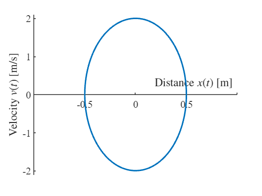
We have noticed the position of a particular nice motorcycle
Plot its velocity and acceleration curves for !
syms t
x = piecewise(0 <= t < 10, t^2,...
t >= 10, 20*t-100)Now we just differentiate
x_dot = diff(x,t)x_ddot = diff(x,t,2)figure;
fplot(x,[0,30],'b','Linewidth',2)
xlabel('Time [s]')
ylabel('Distance [m]')
title('Distance')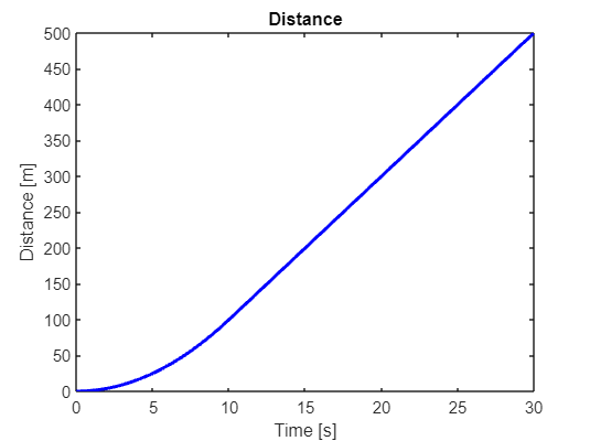
figure;
fplot(x_dot,[0,30],'r','Linewidth',2)
xlabel('Time [s]')
ylabel('Velocity [m]')
title('Velocity')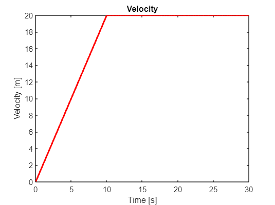
figure;
fplot(x_ddot,[0,30],'m','Linewidth',2)
xlabel('Time [s]')
ylabel('Acceleration [m]')
title('Acceleration')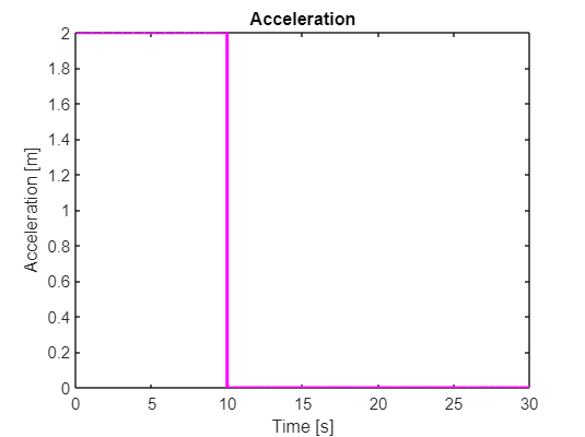
A sports car manufacturer is limiting the power for one of the models by limiting the fuel consumption when the throttle is fully engaged such that the acceleration at any moment is proportional with the constant with respect to the difference in wanted top speed and the current speed . Assume the car starts from rest and the driver puts the pedal to the metal.
Draw the distance and velocity curve
How long does is take to reach top speed and how far has the car traveled?
What is the 0-100 km/h time and distance?
Solution:
From the problem description we create the model using the ODE:
clear
syms x(t)
x_dot = diff(x,t)v_1 = 80; k = 0.1;
DE = diff(x,t,2) == k*(v_1-x_dot)IV = [x_dot(0)==0, x(0)==0]x = dsolve(DE,IV)v = diff(x,t)figure;
fplot(v*3.6, [0,70], 'Linewidth',2)
xlabel('Time [s]')
ylabel('Velocity [m/s]')
axis([0,70,0,300])
hold on
fplot(100, [0,70],'b--')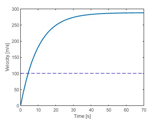
vn = matlabFunction(v);

v_max = limit(v*3.6, t, inf)vn(70)*3.6ans = 287.7374s1 = double(int(v,0,70))s1 = 4.8007e+03The car reaches a maximum theoretical speed of 288 km/h which takes around 70 seconds and the car has then traveled around 4.8 km.
syms t positive
t100 = double(solve(v*3.6==100,t))
t100 = 4.2652double(int(v,0,t100))ans = 63.4370The car reaches 100 km/h after 4.27 seconds, not great, not terrible either, by then the car has traveled around 63 meters.
x_i = 0;
x_dot_i = 0;
ti = 0;
dt = 0.1;

t1 = 70;
n = length(0:dt:t1)
n = 701x = NaN(n,1);
t =(0:dt:t1)';
x_dot = x;
fprintf('i | t | x_dot | x_i')
fprintf('------------------------------')
i = 1;
while ti <= t1
ti = ti + dt;
x_dot_i = x_dot_i + 0.1*(80-x_dot_i)*dt;
x_i = x_i + x_dot_i*dt;
fprintf('%d | %0.2f | %0.4f | %0.4f \n',i,ti,x_dot_i, x_i)
t(i) = ti;
x(i) = x_i;
x_dot(i) = x_dot_i;
i = i+1;
endi | t | x_dot | x_i
------------------------------
1 | 0.10 | 0.8000 | 0.0800
2 | 0.20 | 1.5920 | 0.2392
3 | 0.30 | 2.3761 | 0.4768
4 | 0.40 | 3.1523 | 0.7920
5 | 0.50 | 3.9208 | 1.1841
6 | 0.60 | 4.6816 | 1.6523
7 | 0.70 | 5.4348 | 2.1958
...
698 | 69.80 | 79.9281 | 4792.7114
699 | 69.90 | 79.9289 | 4800.7042
700 | 70.00 | 79.9296 | 4808.6972figure;
plot(t,x,'b-','Linewidth',2)
xlabel('Time [s]')
ylabel('Distance [m]')
title('Numerical solution')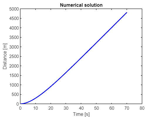
figure;
plot(t,x_dot,'r-','Linewidth',2)
xlabel('Time [s]')
ylabel('Velocity [m/s]')
title('Numerical solution')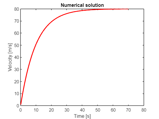
The curvilinear motion of a particle is defined by and , where is in meter per second, is in meters and is in seconds. It is also known that when . Plot the path of the particle and determine its velocity and acceleration when the position is reached.
clear
syms x(t) y(t)
syms t positive

y = 100 - 4*t^2DE = diff(x,t) == 50 - 16*tBV = x(0) == 0x = dsolve(DE,BV)t_y0 = solve(y==0,t)figure
fplot(x,y,[0,double(t_y0)],'Linewidth',2)
grid on
xlabel('$x(t)$ [m]','Interpreter','latex');
ylabel('$y(t)$ [m]','Interpreter','latex');
axis equal
title("The path of the particle")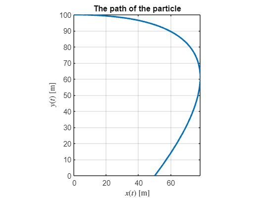
Now we can compute the velocity and acceleration, first simply in Cartesian coordinates
r = [x,y].'r_dot = diff(r,t)r_ddot = diff(r,t,2)Velocity when
r_dot_y0 = subs(r_dot, t, t_y0)t1 = double(t_y0);
figure; hold on
fplot(x,y,[0,t1],'Linewidth',2)
grid on
xlabel('$x(t)$ [m]','Interpreter','latex');
ylabel('$y(t)$ [m]','Interpreter','latex');
axis equal
title("The path of the particle")
xn = matlabFunction(x);
yn = matlabFunction(y);
v = matlabFunction(r_dot);
a = double(r_ddot)a = 2x1
-16
-8t = 0;
vi = v(t);
xi = xn(t);
yi = yn(t);
plot(xn(0),yn(0),'ko','MarkerFacecolor','k','MarkerSize',4)
text(xn(0),yn(0)+5,'$t=0$','Interpreter','latex')
plot(xn(1),yn(1),'ko','MarkerFacecolor','k','MarkerSize',4)
text(xn(1)-10,yn(1)-5,'$t=1$','Interpreter','latex')
plot(xn(2),yn(2),'ko','MarkerFacecolor','k','MarkerSize',4)
text(xn(2)-15,yn(2)-5,'$t=2$','Interpreter','latex')
plot(xn(3),yn(3),'ko','MarkerFacecolor','k','MarkerSize',4)
text(xn(3)-18,yn(3)-1,'$t=3$','Interpreter','latex')
plot(xn(4),yn(4),'ko','MarkerFacecolor','k','MarkerSize',4)
text(xn(4)-18,yn(4)-1,'$t=4$','Interpreter','latex')
plot(xn(5),yn(5),'ko','MarkerFacecolor','k','MarkerSize',4)
text(xn(5)+5,yn(5)-1,'$t=5$','Interpreter','latex')
hqv = quiver(xi, yi, vi(1), vi(2), 1,'b');
hqa = quiver(xi, yi, a(1), a(2), 1,'r');
hp = plot(xi,yi,'ko','MarkerFacecolor','k');
axis([-10,100,-45,110])% for t = linspace(0,t1,100)
% vi = v(t);
% xi = xn(t);
% yi = yn(t);
% set(hp,'XData',xi,'Ydata',yi)
% set(hqv,'XData',xi,'Ydata',yi,'UData',vi(1),'VData',vi(2))
% set(hqa,'XData',xi,'Ydata',yi,'UData',a(1),'VData',a(2))
% drawnow
% end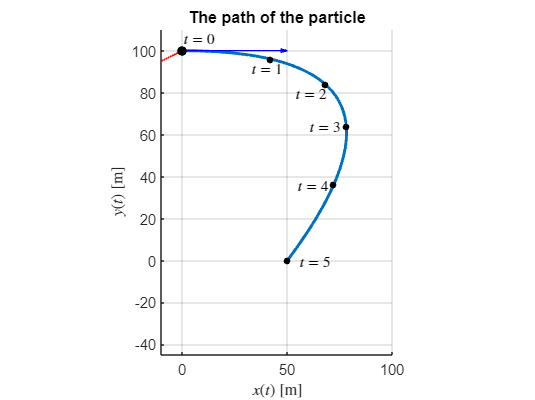
We note that the acceleration is constant in this perticular examples, which is due to the velocity constraint in the x-direction.

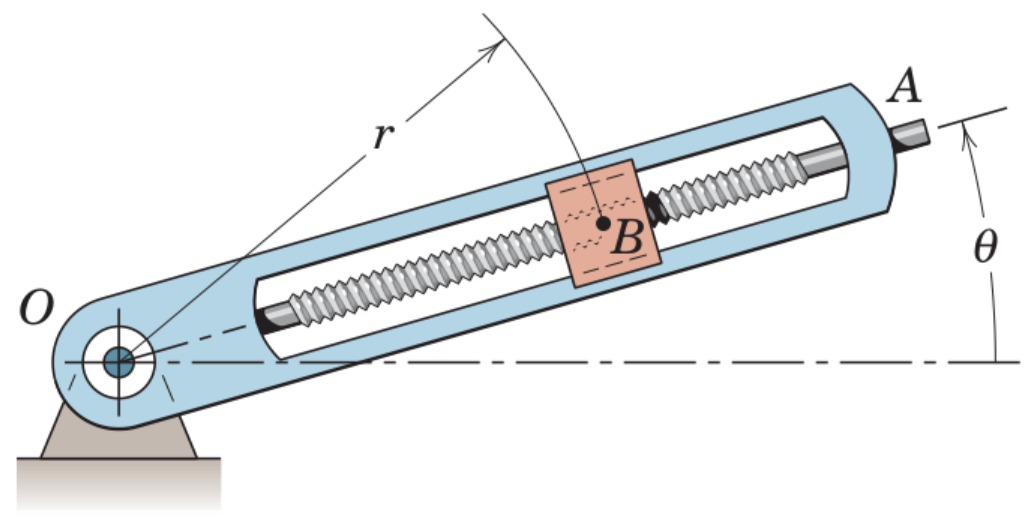
The motion of a particle, , confined to the radial screw of an arm is to be studied. Let and and analyse the motion of the particle in Cartesian and polar coordinates!
We begin by expressing the particles position
clear

syms theta(t) r(t)

rr = r*[cos(theta), sin(theta)].'Then we let matlab compute the derivatives
rr_dot = diff(rr,t);
syms r_dot theta_dot r_ddot theta_ddot
rr_dot = subs(rr_dot, [diff(r,t), diff(theta,t)], [r_dot,theta_dot])rr_ddot = diff(rr,t,2);
rr_ddot = subs(rr_ddot, [diff(r,t,2), diff(theta,t,2)], ...
[r_ddot, theta_ddot]);
rr_ddot = subs(rr_ddot, [diff(r,t), diff(theta,t)], ...
[r_dot, theta_dot])In the above expressions, we made the derivatives easier to read by converting to Newtonian notation. Clearly, Matlab can handle tedious derivation.
Now, we define the polar bases
e_r = [cos(theta), sin(theta)].';
e_theta = [-sin(theta), cos(theta)].';
where is orthogonal according to the right-hand rule (rotate 90 degrees counter clockwise).
Now just project the Cartesial vectors onto the polar bases. We can get away with the "low budget" projection since the bases have unit length, i.e., . We recall that the dot product is just a matrix multiplication
r_dot_rtheta = simplify([rr_dot.'*e_r, rr_dot.'*e_theta])r_ddot_rtheta = simplify([rr_ddot.'*e_r, rr_ddot.'*e_theta])We can see that we end up with the same expressions as we have tediously derived using the classical approach in the sections above.
Now, let and and create plots over the situation.
syms t
theta = 0.2*t+0.02*t^3;
r = 0.2 + 0.04*t^2;
rr = r*[cos(theta), sin(theta)].';
x = rr(1)y = rr(2)xn = matlabFunction(x);
yn = matlabFunction(y);
figure
fplot(rr(1), rr(2), [0,5], 'LineWidth', 2)
axis equal
grid on
xlabel('$x(t)$ [m]','Interpreter','latex');
ylabel('$y(t)$ [m]','Interpreter','latex');
title("The path of the particle")
axis([-1.3,0.5,-0.5,0.8])
text(xn(1),yn(1),'$t=1$','Interpreter','latex','Backgroundcolor','w')
text(xn(2),yn(2),'$t=2$','Interpreter','latex','Backgroundcolor','w')
text(xn(3),yn(3),'$t=3$','Interpreter','latex','Backgroundcolor','w')
text(xn(4),yn(4),'$t=4$','Interpreter','latex','Backgroundcolor','w')
text(xn(5),yn(5),'$t=5$','Interpreter','latex','Backgroundcolor','w')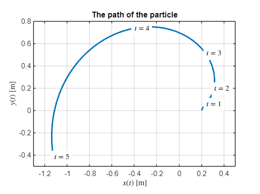
figure; hold on;
fplot(diff(x,t),[0,5],'LineWidth', 2,'DisplayName','$\dot x$')
fplot(diff(y,t),[0,5],'LineWidth', 2,'DisplayName','$\dot y$')
fplot(diff(x,t,2),[0,5],'LineWidth', 2,'DisplayName','$\ddot x$')
fplot(diff(y,t,2),[0,5],'LineWidth', 2,'DisplayName','$\ddot y$')
legend('show','Interpreter','latex')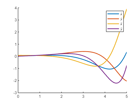
syms t
xy_dot = matlabFunction( simplify(diff([x,y],t)) );
xy_ddot = matlabFunction( simplify(diff([x,y],t,2)) );

figure; hold on
fplot(rr(1), rr(2), [0,5], 'LineWidth', 2)
axis equal
grid on
xlabel('$x(t)$ [m]','Interpreter','latex');
ylabel('$y(t)$ [m]','Interpreter','latex');
title("The path of the particle")
axis([-1.5,0.7,-0.5,1.3])

t = 1;
vi = xy_dot(t);
ai = xy_ddot(t);
xi = xn(t);
yi = yn(t);
hp = plot([0,xn(t)],[0,yn(t)],'k-');
hv = quiver(xi, yi, vi(1), vi(2),0.4,'b');
ha = quiver(xi, yi, ai(1), ai(2),0.4,'r');
for t = linspace(0,5,200)
vi = xy_dot(t);
ai = xy_ddot(t);
xi = xn(t);
yi = yn(t);
set(hp,'XData',xi,'Ydata',yi)
set(hv,'XData',xi,'Ydata',yi,'UData',vi(1),'VData',vi(2))
set(ha,'XData',xi,'Ydata',yi,'UData',ai(1),'VData',ai(2))
drawnow
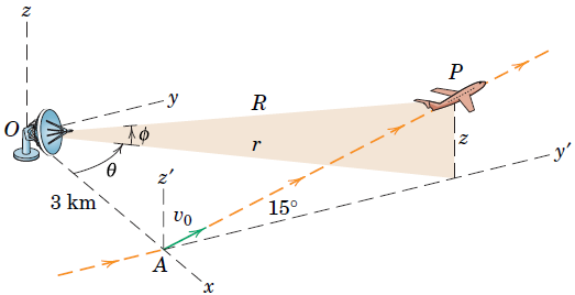
endAn aircraft takes off at with a velocity of 250 km/h and climbs in the vertical plane at the constant angle with an acceleration along its flight path of . The flight progress is monitored by radar at point .
Determine the velocity of the aircraft in cylindrical coordinates 60 seconds after takeoff and find .
Determine the velocity in spherical coordinates 60 seconds after takeoff and find .
clear
syms t positive
syms y(t) z(t)

v0 = 250/3.6;
alpha = 15*pi/180;
a = 0.8;

OA = [3000; 0; 0];
eAP = [0; cos(alpha); sin(alpha)];
V0 = v0*eAP;
Acc = a*eAP;

x = 3000;

yp = diff(y,1);
ypp = diff(y,2);
DEy = ypp == Acc(2);
BVy = [yp(0) == V0(2); y(0) == 0];
y = vpa(dsolve(DEy,BVy), 4)zp = diff(z,1);
zpp = diff(z,2);
DEz = zpp == Acc(3);
BVz = [zp(0) == V0(3); z(0) == 0];
z = vpa(dsolve(DEz,BVz), 4)R = vpa([x; y; z],4)Rp = vpa(diff(R,1),4)Rpp = vpa(diff(R,2),4)The situation graphically
figure; hold on; grid on; axis equal
plot3(subs(R(1),t,0),subs(R(2),t,0),subs(R(3),t,0),'ob', 'Displayname',"start")
fplot3(R(1),R(2),R(3),[0,60],'-b', 'Displayname',"path")
plot3([0,4000], [0,0], [0,0], '--k', 'HandleVisibility','off')
plot3([0,0], [0,4000], [0,0], '--k', 'HandleVisibility','off')
plot3([0,0], [0,0], [0,4000], '--k', 'HandleVisibility','off')
plot3(subs(R(1),t,60),subs(R(2),t,60),subs(R(3),t,60),'or', 'Displayname',"$t=60$s")
plot3(0,0,0,'ok', 'HandleVisibility','off')
quiver3(subs(R(1),t,60),subs(R(2),t,60),subs(R(3),t,60),subs(Rp(1),t,60),subs(Rp(2),t,60),subs(Rp(3),t,60),15,'k','LineWidth', 1, 'Displayname',"velocity")
quiver3(subs(R(1),t,60),subs(R(2),t,60),subs(R(3),t,60),0,subs(Rp(2),t,60),0,15,'g','LineWidth', 1, 'Displayname',"y-velocity")
quiver3(subs(R(1),t,60),subs(R(2),t,60),subs(R(3),t,60),0,0,subs(Rp(3),t,60),15,'b','LineWidth', 1, 'Displayname',"z-velocity")
view([43 23])
xlabel('x')
ylabel('y')
zlabel('z')
legend("show","location","northwest",Interpreter="latex")
title('Velocity in cartesian coordinates')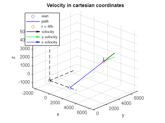
Cylindrical coordinates
OP_xy = [x; y; 0];
eOP_xy = OP_xy/(sqrt(x^2 + y^2));
r_cyl = sqrt(x^2 + y^2);
theta = atan(y/x);
rp_cyl = diff(r_cyl);
thetap = diff(theta);
Rp_cyl = rp_cyl * eOP_xy;
Theta_p = thetap * [0;0;1];
Tan_p = cross(Theta_p,r_cyl*eOP_xy);

rp_cyl_60 = vpa(subs(rp_cyl,t,60),5)
rp_cyl_60 = 99.234thetap_60 = vpa(subs(thetap,t,60),5)thetap_60 = 0.0088791zp_60 = vpa(subs(Rp(3),t,60),5)zp_60 = 30.397figure
hold on
grid on
axis equal
plot3(subs(R(1),t,0),subs(R(2),t,0),subs(R(3),t,0),'ob', 'Displayname',"start")
fplot3(R(1),R(2),R(3),[0,60],'-b', 'Displayname',"path")
plot3([0,4000], [0,0], [0,0], '--k', 'HandleVisibility','off')
plot3([0,0], [0,4000], [0,0], '--k', 'HandleVisibility','off')
plot3([0,0], [0,0], [0,4000], '--k', 'HandleVisibility','off')
plot3(subs(R(1),t,60),subs(R(2),t,60),subs(R(3),t,60),'or', 'Displayname',"$t=60$s")
plot3(0,0,0,'ok', 'HandleVisibility','off')
quiver3(subs(R(1),t,60),subs(R(2),t,60),subs(R(3),t,60),subs(Rp(1),t,60),subs(Rp(2),t,60),subs(Rp(3),t,60),15,'k','LineWidth', 1, 'Displayname',"$V$")
quiver3(subs(R(1),t,60),subs(R(2),t,60),subs(R(3),t,60),subs(Rp_cyl(1),t,60),subs(Rp_cyl(2),t,60),subs(Rp_cyl(3),t,60),15,'r','LineWidth', 1, 'Displayname',"$V_r$")
quiver3(subs(R(1),t,60),subs(R(2),t,60),subs(R(3),t,60),subs(Tan_p(1),t,60),subs(Tan_p(2),t,60),subs(Tan_p(3),t,60),15,'g','LineWidth', 1, 'Displayname',"$V_\theta$")
quiver3(subs(R(1),t,60),subs(R(2),t,60),subs(R(3),t,60),0,0,subs(Rp(3),t,60),15,'b','LineWidth', 1, 'Displayname',"$V_z$")
view([43 23])
xlabel('x');ylabel('y');zlabel('z')
legend("show","location","northwest",Interpreter="latex")
title('Velocity in cylindrical coordinates')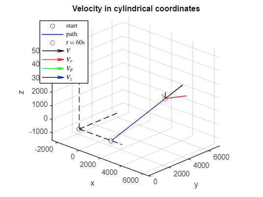
Spherical coordinates
r_sph = sqrt(x^2 + y^2 + z^2);
OP = [x; y; z];
eOP = OP/r_sph;
phi = atan(z/r_sph);
rp_sph = diff(r_sph);
phip = diff(phi);
Rp_sph = rp_sph * eOP;
Phi_p = phip * cross(eOP,[0;0;1]);
Phi_tan_p = cross(Phi_p,r_sph*eOP);
Tan_p = cross(Theta_p,r_sph*eOP);

rp_sph_60 = vpa(subs(rp_sph,t,60),5)thetap_60 = vpa(subs(thetap,t,60),5)phip_60 = vpa(subs(phip,t,60),5)figure; hold on; grid on; axis equal
plot3(subs(R(1),t,0),subs(R(2),t,0),subs(R(3),t,0),'ob', 'Displayname',"start")
fplot3(R(1),R(2),R(3),[0,60],'-b', 'Displayname',"path")
plot3([0,4000], [0,0], [0,0], '--k', 'HandleVisibility','off')
plot3([0,0], [0,4000], [0,0], '--k', 'HandleVisibility','off')
plot3([0,0], [0,0], [0,4000], '--k', 'HandleVisibility','off')
plot3(subs(R(1),t,60),subs(R(2),t,60),subs(R(3),t,60),'or', 'Displayname',"$t=60$s")
plot3(0,0,0,'ok', 'HandleVisibility','off')
quiver3(subs(R(1),t,60),subs(R(2),t,60),subs(R(3),t,60),subs(Rp(1),t,60),subs(Rp(2),t,60),subs(Rp(3),t,60),15,'k','LineWidth', 1, 'Displayname',"$V$")
quiver3(subs(R(1),t,60),subs(R(2),t,60),subs(R(3),t,60),subs(Rp_sph(1),t,60),subs(Rp_sph(2),t,60),subs(Rp_sph(3),t,60),15,'r','LineWidth', 1, 'Displayname',"$V_r$")
quiver3(subs(R(1),t,60),subs(R(2),t,60),subs(R(3),t,60),subs(Tan_p(1),t,60),subs(Tan_p(2),t,60),subs(Tan_p(3),t,60),15,'g','LineWidth', 1, 'Displayname',"$V_\theta$")
quiver3(subs(R(1),t,60),subs(R(2),t,60),subs(R(3),t,60),subs(Phi_tan_p(1),t,60),subs(Phi_tan_p(2),t,60),subs(Phi_tan_p(3),t,60),100,'b','LineWidth', 1, 'Displayname',"$V_\phi$")
view([43 23])
xlabel('x'); ylabel('y'); zlabel('z')
legend("show","location","northwest",Interpreter="latex")
title('Velocity in spherical coordinates')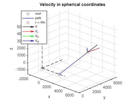
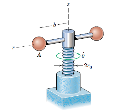
The power screw starts from rest and is given a rotational speed which increases uniformly with time according to , where is constant. Determine the velocity and acceleration of the center of ball when the screw has turned through one complete revolution from rest. The lead of the screw (advancement per revolution) is .
clear
syms t positive
syms theta(t) r(t)
Let , and .
k = 2;
r0 = 20;
L = 3;
theta_p = diff(theta)DE = theta_p == k*tBV = theta(0)==0theta = dsolve(DE,BV)t1 = double( max(solve(theta==2*pi,t)) )t1 = 2.5066x = cos(theta)*r0y = sin(theta)*r0z = -theta*L/(2*pi)Rp = diff([x;y;z])Rpp = diff([x;y;z],2)Rn = matlabFunction([x;y;z]);
Rpn = matlabFunction(Rp);
Rppn = matlabFunction(Rpp);
Ri = Rn(t1)Ri = 3x1
20.0000
0.0000
-3.0000Rpi = Rpn(t1)Rpi = 3x1
-0.0000
100.2651
-2.3937Rppi = Rppn(t1)Rppi = 3x1
-502.6548
40.0000
-0.9549figure; hold on; grid on; axis equal
fplot3(x,y,z,[0,4], 'Displayname',"path")
plot3(r0,0,0,'ok', 'Displayname',"starting point")
hp = plot3(Ri(1),Ri(2),Ri(3),'ob', 'Displayname',"$\theta=2\pi$");
hqv = quiver3(Ri(1),Ri(2),Ri(3),Rpi(1),Rpi(2),Rpi(3),0.1,'b','LineWidth', 2, 'Displayname',"velocity");
hqa = quiver3(Ri(1),Ri(2),Ri(3),Rppi(1),Rppi(2),Rppi(3),0.02,'r','LineWidth', 2, 'Displayname',"acceleration");
view([48.4 31.5])
xlabel('x'); ylabel('y'); zlabel('z')
legend("show","location","northwest",Interpreter="latex")
axis([-25,25,-25,25,-25,25])for ti = linspace(0,4,100)
Ri = Rn(ti);
Rpi = Rpn(ti);
Rppi = Rppn(ti);
set(hp,'XData',Ri(1), 'YData', Ri(2), 'Zdata', Ri(3))
set(hqv,'XData',Ri(1), 'YData', Ri(2), 'Zdata', Ri(3), 'UData', Rpi(1), 'VData', Rpi(2), 'WData', Rpi(3))
set(hqa,'XData',Ri(1), 'YData', Ri(2), 'Zdata', Ri(3), 'UData', Rppi(1), 'VData', Rppi(2), 'WData', Rppi(3))
drawnow
end
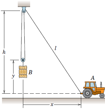
A tractor is used to hoist the bale using a pulley arrangement as shown. If the tractor at has a forward velocity , determine an expression for the upward velocity
Solution:
This is a so called constrained motion. We can tackle this problem by finding the geometric relation between and . We take note of a triangle and thus utilize the Pythagorean theorem to formulate
Also, we note the geometry of the rope, which has a constant length .
clear
syms l(t) h x(t) y(t) L

ekv = [x^2 + h^2 == l^2
       L == 2*(h-y) + l];
ekv = [ekv; diff(ekv,t)];
Cleaning up the output and simplifying
syms l_dot v_A v_B positive
ekv = subs(ekv, [diff(x,t), diff(y,t), diff(l,t)], [v_A, v_B, l_dot]);

ekv = subs(ekv,[x,y,l],[sym('x'), sym('y'), sym('l')])syms y l x positive
[y, v_B, l, l_dot] = solve(ekv,[y, v_B, l, l_dot])Warning: Solutions are only valid under certain conditions. To include parameters and conditions in the solution, specify the 'ReturnConditions' value as 'true'.y =
v_B =
l =
l_dot =
Animation
h = 5;
L = 3*h;
r_A = [x;0]r_B = simplify(subs([0;y]))r_C = [0;h]r_C = 2x1
0
5r_A_n = matlabFunction(r_A);
r_B_n = matlabFunction(r_B);
xi = 4;
r_A_i = r_A_n(xi)r_A_i = 2x1
4
0r_B_i = r_B_n(xi)r_B_i = 2x1
0
0.7016x_at_y4 = double(solve(r_B(2)==4,x))x_at_y4 = 12figure; hold on; axis equal;
hAC = plot([r_C(1), r_A_i(1)], [r_C(2), r_A_i(2)], '-ko', ...
'MarkerFaceColor','k','LineWidth',2);
hBC = plot([r_C(1), r_B_i(1)], [r_C(2), r_B_i(2)], '-ko', ...
'MarkerFaceColor','k','LineWidth',2);
htA = text(r_A_i(1)+0.1,r_A_i(2)+0.2,'$A$','interpreter','latex');
text(r_C(1)+0.1,r_C(2)+0.2,'$C$','interpreter','latex');
htB = text(r_B_i(1)+0.1,r_B_i(2)+0.2,'$B$','interpreter','latex');
axis([-1,15,0,5])
for xi = linspace(0,x_at_y4,50)
r_A_i = r_A_n(xi);
r_B_i = r_B_n(xi);
set(hAC,'XData',[r_C(1), r_A_i(1)],'YData',[r_C(2), r_A_i(2)])
set(hBC,'XData',[r_C(1), r_B_i(1)],'YData',[r_C(2), r_B_i(2)])
set(htA,'Position',[r_A_i(1)+0.1,r_A_i(2)+0.2])
set(htB,'Position',[r_B_i(1)+0.1,r_B_i(2)+0.2])
drawnow
end
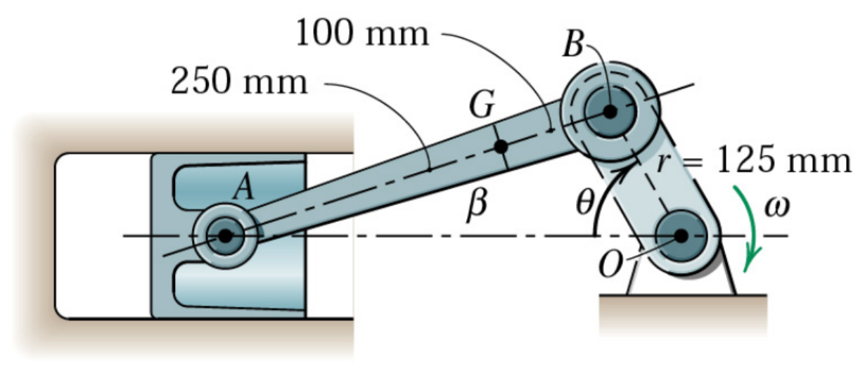
Study the motion of the slider-crank mechanism. Plot the motion of and as well as their velocities and accelerations as a function of . Let the angular velocity rad/s.
Solution:
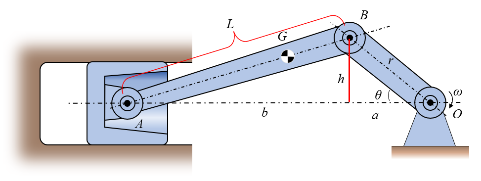
Typical example, we can tackle this using implicit derivation and let Matlab do the heavy lifting. Model the geometry relations first. Let denote the distance . Then we utilize Pythagoras' theorem to formulate the point , using vectors. Let denote the height over the x-axis to point .
clear
syms theta(t)
syms L r positive

h = r*sin(theta);
a = r*cos(theta);
b = sqrt(L^2 - h^2);

r_A = [-(a+b); 0]r_B = r*[-cos(theta); sin(theta)]r_BA = r_A - r_B;
r_G = r_B + 100/(100+250)*r_BAsyms theta_dot theta_ddot positive
r_A_dot = subs(diff(r_A,t), [diff(theta,t), theta], [theta_dot, sym('theta', 'positive')]);
r_A_ddot = subs(diff(r_A,t,2), [diff(theta,t), diff(theta,t,2), theta], ...
[theta_dot, theta_ddot, sym('theta', 'positive')]);
r_A_dot = formula(r_A_dot)r_A_ddot = formula(r_A_ddot)r_B_dot = subs(diff(r_B,t), [diff(theta,t), theta], [theta_dot, sym('theta','positive')]);
r_B_dot = formula(r_B_dot)r_B_dot_m = simplify(norm(r_B_dot))r_B_ddot = subs(diff(r_B,t,2), [diff(theta,t), diff(theta,t,2), theta], ...
[theta_dot, theta_ddot, sym('theta', 'positive')]);
r_B_ddot = formula(r_B_ddot)r_B_ddot_m = simplify(norm(r_B_ddot))r_G_dot = subs(diff(r_G,t), [diff(theta,t), theta], ...
[theta_dot, sym('theta','positive')]);
r_G_dot = formula(r_G_dot)r_G_ddot = subs(diff(r_G,t,2), [diff(theta,t), diff(theta,t,2), theta], ...
[theta_dot, theta_ddot, sym('theta','positive')]);
r_G_ddot = formula(r_G_ddot)Substitute with some numerical data
symData = [L, r, theta_dot, theta_ddot, theta];
numData = [(250+100)/1000, 125/1000, 25*2*pi, 0, sym('theta','positive')];
L = (250+100)/1000; r = 125/1000; theta_dot = 25; theta_ddot = 0;

r_A = subs(r_A);
r_A = subs(r_A,theta,sym('theta','positive'));
r_A = formula(r_A);

r_B = subs(r_B);
r_B = subs(r_B,theta,sym('theta','positive'));
r_B = formula(r_B);

r_G = subs(r_G);
r_G = subs(r_G,theta,sym('theta','positive'));
r_G = formula(r_G)theta = sym('theta','positive');
r_B_dot = subs(r_B_dot);
r_B_ddot = subs(r_B_ddot);
r_A_dot = simplify(subs(r_A_dot));
r_A_ddot = simplify(subs(r_A_ddot));
r_G_dot = simplify(subs(r_G_dot));
r_G_ddot = simplify(subs(r_G_ddot));
r_A_dot_m = norm(r_A_dot);
r_B_dot_m = norm(r_B_dot);
r_G_dot_m = norm(r_G_dot);
r_A_ddot_m = simplify(r_A_ddot(1))r_B_ddot_m = simplify(norm(r_B_ddot))r_G_ddot_m = simplify(norm(r_G_ddot))figure; hold on; grid on
fplot(r_A_dot_m,[0,2*pi],'LineWidth',2,'Displayname','$|\dot \mathbf{r}_A|$')
fplot(r_B_dot_m,[0,2*pi],'LineWidth',2,'Displayname','$|\dot \mathbf{r}_B|$')
fplot(r_G_dot_m,[0,2*pi],'LineWidth',2,'Displayname','$|\dot \mathbf{r}_G|$')
legend('show',interpreter='latex')
tickRangeDegrees = 0:45:360;
xticks(tickRangeDegrees*pi/180);
xticklabels(cellstr(num2str(tickRangeDegrees')));
xlabel('$\theta$ [degrees]',interpreter='latex')
ylabel('Speed [m/s]',interpreter='latex')
title('Crank-slider speed')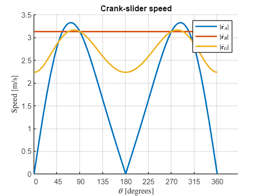
figure; hold on; grid on
fplot(r_A_ddot_m,[0,2*pi],'LineWidth',2,'Displayname','$\ddot r_{Ax}$')
fplot(r_B_ddot_m,[0,2*pi],'LineWidth',2,'Displayname','$|\ddot \mathbf{r}_B|$')
fplot(r_G_ddot_m,[0,2*pi],'LineWidth',2,'Displayname','$|\ddot \mathbf{r}_G|$')
legend('show',interpreter='latex')
tickRangeDegrees = 0:45:360;
xticks(tickRangeDegrees*pi/180);
xticklabels(cellstr(num2str(tickRangeDegrees')));
xlabel('$\theta$ [degrees]',interpreter='latex')
ylabel('Acceleration [$\mathrm{m/s}^2$]',interpreter='latex')
title('Crank-slider acceleration')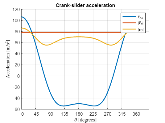
% r_A_n = matlabFunction(r_A);
% r_B_n = matlabFunction(r_B);
% r_G_n = matlabFunction(r_G);
%
% r_A_dot_n = matlabFunction(r_A_dot);
% r_B_dot_n = matlabFunction(r_B_dot);
% r_G_dot_n = matlabFunction(r_G_dot);
%
% r_A_ddot_n = matlabFunction(r_A_ddot);
% r_B_ddot_n = matlabFunction(r_B_ddot);
% r_G_ddot_n = matlabFunction(r_G_ddot);
%
% r_A_dot_m_n = matlabFunction(r_A_dot_m);
% r_B_dot_m_n = matlabFunction(r_B_dot_m);
% r_G_dot_m_n = matlabFunction(r_G_dot_m);
%
% r_A_ddot_m_n = matlabFunction(r_A_ddot_m);
% r_B_ddot_m_n = matlabFunction(r_B_ddot_m);
% r_G_ddot_m_n = matlabFunction(r_G_ddot_m);
%
% theta = 30*pi/180;
%
% r_A_i = r_A_n(theta)*1000;
% r_B_i = r_B_n(theta)*1000;
% r_G_i = r_G_n(theta)*1000;
%
% r_A_dot_i = r_A_dot_n(theta);
% r_B_dot_i = r_B_dot_n(theta);
% r_G_dot_i = r_G_dot_n(theta);
%
% r_A_ddot_i = r_A_ddot_n(theta);
% r_B_ddot_i = r_B_ddot_n(theta);
% r_G_ddot_i = r_G_ddot_n(theta);
%
% xmin = -500; xmax = 150;
% ymin = -150; ymax = 150;
%
% close all
% figure;
% set(gcf,'Visible','on','Color','w','Position',[680   242   872   636])
% subplot(2,2,[1,2])
% hold on; axis equal;
% hB = plot([0,r_B_i(1)],[0,r_B_i(2)],'-ko','MarkerFaceColor','k');
% text(5,-5,'$O$',interpreter='latex')
% plot([xmin,xmax],[0,0],':k')
%
% hAB = plot([r_A_i(1),r_B_i(1)],[r_A_i(2),r_B_i(2)],'-ko','MarkerFaceColor','k');
%
%
%
% scale_v = 20;
% scale_a = 1;
% hqBv = quiver(r_B_i(1), r_B_i(2), r_B_dot_i(1), r_B_dot_i(2), scale_v, 'b', 'LineWidth',2);
% hqBa = quiver(r_B_i(1), r_B_i(2), r_B_ddot_i(1), r_B_ddot_i(2), scale_a, 'r', 'LineWidth',2);
% hqAv = quiver(r_A_i(1), r_A_i(2), r_A_dot_i(1), r_A_dot_i(2), scale_v, 'b', 'LineWidth',2);
% hqAa = quiver(r_A_i(1), r_A_i(2), r_A_ddot_i(1), r_A_ddot_i(2), scale_a, 'r', 'LineWidth',2);
% hqGv = quiver(r_G_i(1), r_G_i(2), r_G_dot_i(1), r_G_dot_i(2), scale_v, 'b', 'LineWidth',2);
% hqGa = quiver(r_G_i(1), r_G_i(2), r_G_ddot_i(1), r_G_ddot_i(2), scale_a, 'r', 'LineWidth',2);
%
% htG = text(r_G_i(1)+5,r_G_i(2)-5, '$G$', interpreter='latex');
% hG = plot(r_G_i(1),r_G_i(2),'ko','MarkerFaceColor','k');
% htA = text(r_A_i(1)+5,r_A_i(2)-5, '$A$', interpreter='latex');
% htB = text(r_B_i(1)+5,r_B_i(2)-5, '$B$', interpreter='latex');
%
% axis([xmin, xmax, ymin, ymax])
% xlabel('$x$', interpreter='latex'); ylabel('$y$', interpreter='latex')
%
% htitle = title(['$\theta=$',num2str(theta*180/pi),'$^\circ$'], interpreter='latex');
%
% subplot(2,2,[3]); hold on; grid on
% fplot(r_A_dot_m,[0,2*pi],'LineWidth',2,'Displayname','$|\dot \mathbf{r}_A|$')
% fplot(r_B_dot_m,[0,2*pi],'LineWidth',2,'Displayname','$|\dot \mathbf{r}_B|$')
% fplot(r_G_dot_m,[0,2*pi],'LineWidth',2,'Displayname','$|\dot \mathbf{r}_G|$')
% legend('show','interpreter','latex','Position',[0.17282 0.44296 0.21282 0.02450],...
%     'Orientation','horizontal')
% tickRangeDegrees = 0:45:360;
% xticks(tickRangeDegrees*pi/180);
% xticklabels(cellstr(num2str(tickRangeDegrees')));
% xlabel('$\theta$ [degrees]',interpreter='latex')
% ylabel('Speed [m/s]',interpreter='latex')
%
% c1 = [0 0.4470 0.7410];
% c2 = [0.8500 0.3250 0.0980];
% c3 = [0.9290 0.6940 0.1250];
% hpAv = plot(theta, r_A_dot_m_n(theta),'o','color',c1,'MarkerFaceColor',c1,'HandleVisibility','off');
% hpBv = plot(theta, r_B_dot_m_n(theta),'o','color',c2,'MarkerFaceColor',c2,'HandleVisibility','off');
% hpGv = plot(theta, r_G_dot_m_n(theta),'o','color',c3,'MarkerFaceColor',c3,'HandleVisibility','off');
%
% subplot(2,2,[4]); hold on; grid on
% fplot(r_A_ddot_m,[0,2*pi],'LineWidth',2,'Displayname','$\ddot r_{Ax}$')
% fplot(r_B_ddot_m,[0,2*pi],'LineWidth',2,'Displayname','$|\ddot \mathbf{r}_B|$')
% fplot(r_G_ddot_m,[0,2*pi],'LineWidth',2,'Displayname','$|\ddot \mathbf{r}_G|$')
% legend('show','interpreter','latex','Position',[0.60686 0.44296 0.21282 0.02450],...
%     'Orientation','horizontal')
% tickRangeDegrees = 0:45:360;
% xticks(tickRangeDegrees*pi/180);
% xticklabels(cellstr(num2str(tickRangeDegrees')));
% xlabel('$\theta$ [degrees]',interpreter='latex')
% ylabel('Acceleration [$\mathrm{m/s}^2$]',interpreter='latex')
% hpAa = plot(theta, r_A_ddot_m_n(theta),'o','color',c1,'MarkerFaceColor',c1,'HandleVisibility','off');
% hpBa = plot(theta, r_B_ddot_m_n(),'o','color',c2,'MarkerFaceColor',c2,'HandleVisibility','off');
% hpGa = plot(theta, r_G_ddot_m_n(theta),'o','color',c3,'MarkerFaceColor',c3,'HandleVisibility','off');
%
%
% for theta = linspace(0,2*pi, 100)
%     if theta == 0
%         exportgraphics(gcf,"crank-slider.gif","Append",false)
%     end
%     r_A_i = r_A_n(theta)*1000;
%     r_B_i = r_B_n(theta)*1000;
%     r_G_i = r_G_n(theta)*1000;
%
%     r_A_dot_i = r_A_dot_n(theta);
%     r_B_dot_i = r_B_dot_n(theta);
%     r_G_dot_i = r_G_dot_n(theta);
%
%     r_A_ddot_i = r_A_ddot_n(theta);
%     r_B_ddot_i = r_B_ddot_n(theta);
%     r_G_ddot_i = r_G_ddot_n(theta);
%
%     set(hAB,'XData', [r_A_i(1),r_B_i(1)], 'Ydata', [r_A_i(2),r_B_i(2)])
%     set(hB,'XData', [0,r_B_i(1)], 'Ydata', [0,r_B_i(2)])
%     set(hG, 'XData', r_G_i(1), 'YData', r_G_i(2))
%     set(htG,'Position',[r_G_i(1)+5,r_G_i(2)-5])
%     set(htA,'Position',[r_A_i(1)+5,r_A_i(2)-5])
%     set(htB,'Position',[r_B_i(1)+5,r_B_i(2)-5])
%     set(htitle,'String', ['$\theta=$',sprintf('%0.0f',theta*180/pi),'$^\circ$'])
%     set(hqBv,'XData',r_B_i(1),'Ydata',r_B_i(2),'Udata',r_B_dot_i(1),'VData',r_B_dot_i(2))
%     set(hqBa,'XData',r_B_i(1),'Ydata',r_B_i(2),'Udata',r_B_ddot_i(1),'VData',r_B_ddot_i(2))
%     set(hqAv,'XData',r_A_i(1),'Ydata',r_A_i(2),'Udata',r_A_dot_i(1),'VData',r_A_dot_i(2))
%     set(hqAa,'XData',r_A_i(1),'Ydata',r_A_i(2),'Udata',r_A_ddot_i(1),'VData',r_A_ddot_i(2))
%     set(hqGv,'XData',r_G_i(1),'Ydata',r_G_i(2),'Udata',r_G_dot_i(1),'VData',r_G_dot_i(2))
%     set(hqGa,'XData',r_G_i(1),'Ydata',r_G_i(2),'Udata',r_G_ddot_i(1),'VData',r_G_ddot_i(2))
%
%     set(hpAv,'XData',theta,'Ydata',r_A_dot_m_n(theta))
%     set(hpBv,'XData',theta,'Ydata',r_B_dot_m_n(theta))
%     set(hpGv,'XData',theta,'Ydata',r_G_dot_m_n(theta))
%     set(hpAa,'XData',theta,'Ydata',r_A_ddot_m_n(theta))
%     set(hpBa,'XData',theta,'Ydata',r_B_ddot_m_n())
%     set(hpGa,'XData',theta,'Ydata',r_G_ddot_m_n(theta))
%
%     exportgraphics(gcf,"crank-slider.gif","Append",true)
%     drawnow
% end