Table of contents
The method for solving problems in kinetics is an extension from statics and the methods used in the corresponding sections. Kinetics is the study of relations between forces and accelerations and a starting point is Newton's equation of motion
where is the center of mass (COM) of a body (or particle). For completeness we shall here state the complete generalized equations of motion extended by Euler et al.
where is the angular moment of inertia for the body at the center of mass, otherwise known as the rotational inertia of a rigid body. We shall give a proper introduction of this quantity in the section of rigid body kinetics. Note that the moment of inertia is given by the geometric relation
where is the vector from the center of rotation (which in this case is the COM) and all infinitesimal points on the body.
Notice that in this general formulation we have and , thus six equations (ODEs) per component, where for each component we derive these equations by the use of a free body diagram, exactly as in statics. In order to get a specific solution to the system of equations we need corresponding initial conditions and/or boundary conditions.
Suffice to say for now, if the body has near zero size, then and we can assume particle dynamics and disregard the rotational part of the equation of motion, resulting in only three degrees of freedom instead of six. Similarly if the rotational acceleration is sufficiently low, we can assume particle dynamics. We will revisit the generalized equations of motion in rigid body kinetics.
Note that Newtons second law of motion does not explicitly relate force to acceleration, but rather momentum, paraphrased: "The time rate of change of a bodies momentum equals the force acting upon it" i.e.,
Thus, we can create models where the body has a change of mass, e.g., rockets. When a body has constant mass the expression reduces to what we are familiar with.
The solution of the equations of motion is typically done by solving a differential equation using either a symbolic or numerical solver. In traditional courses on classical mechanics, countless chapters are spent on deriving various analytical methods and formulas for simplifying problems or solving problems specifically designed to be solved using simple hand calculations. We shall here instead focus on solving problems completely, and be explicit with the visualization of the whole motion.
We can apply two main methods for solving and analyzing dynamics problems. Transient, meaning we formulate an ODE and solve it either analytically of numerically. This gives us the position, velocity and acceleration vectors as a function of time over the complete time frame of interest. For situations where we are interested in solutions only at a particular time (or state) we can formulate the problem as an energy equation instead using Lagrangian or Hamiltonian formulation of mechanics. This can simplify the calculations drastically, since we do not need to iterate to the state from the initial state (using a numerical method) nor determine the accelerations or include forces that do no work.
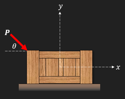
A box is being pushed from rest.
How much force is required to accelerate the box to ?
What is the velocity of the box after seconds?
How far does the box glide? At which time does it come to a stop?
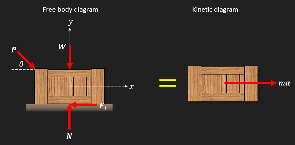
From the figure we get
and the the acceleration vector is
Using Newtons second law of motion we can formulate
clear

syms mu_k m g v_0 P theta N a_x
F_ext = P*[cos(theta); -sin(theta)];
F_N = [0; N];
F_W = [0; -m*g];
F_f = [-mu_k*N; 0];
a = [a_x; 0];

ekv = F_ext + F_N + F_W + F_f == m*aFrom this equation system we need to solve for the same amount of unknowns as we have number of equations, we choose , of course, and for the additional unknown. This is typical in mechanics to get additional unknowns, usually contact forces, or reaction forces. The choice is based on careful analysis of what is considered input parameter and what is an unknown quantity.
[a_x, N] = solve(ekv, [a_x, N])From the expression we can see that the vertical component of causes additional friction in the negative x-direction whereas the horizontal component gives rise to an acceleration in the positive x-direction. Analyzing symbolic expressions before substitution is a good idea in the modeling stage, since we can verify the model much easier.
Let us assume that the box is given a push from during a short time. Let
syms t
P_const = piecewise(t<0.3, 4000, ...
                    t>0.3 , 0)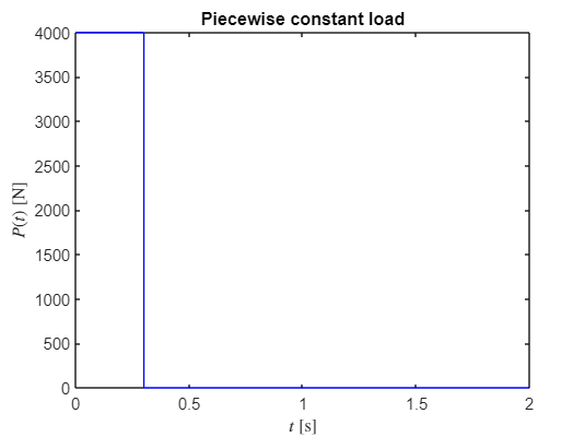
In order to solve this problem we need to tackle this piecewise, we need to set up a differential equation with initial values for the range s and another differential equation with initial values for the range .
We can then formulate the differential equation and solve it to get the position which we can differentiate to get .
Then we can find out at what time the velocity is zero, , it is at this time that the box has come to stop.
We formulate the differential equation in general by
Now, we shall use some numerical values for brevity.
m=50; mu_k=0.3; g = 9.82; theta = 0*pi/180;a_x = subs(a_x)We split the solution into before and after .
For we have
syms x(t)
DE1 = diff(x,t,2) == a_xx_dot = diff(x,t);
BV1 = [x(0) == 0, x_dot(0) == 0];
x1(t) = dsolve(DE1,BV1)x1(t) = subs(x1, P, 4000)v1(t) = diff(x1,t)For we have that
DE2 = vpa(diff(x,t,2) == subs(a_x,P,0) ,2)t1 = 0.3;
BV2 = vpa([x(t1) == x1(t1), x_dot(t1) == v1(t1)],2)x2(t) = dsolve(DE1,BV2);
x2 = vpa(x2,2)v2(t) = diff(x2,t);
v2 = vpa(v2,2)To get the time where the box stops gliding
t2 = double(solve(v2==0, t))t2 = 8.1466x_max = double(x2(t2))x_max = 94.1597Now we can plot the situation!
figure; hold on
fplot(x1,[0,t1],'Linewidth',2)
fplot(x2,[t1,t2],'Linewidth',2)
xlabel('$t$','interpreter','latex')
ylabel('$x(t)$','interpreter','latex')
title('Position of the box')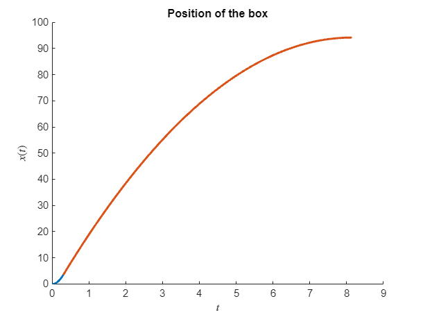
figure; hold on
fplot(v1,[0,t1],'Linewidth',2)
fplot(v2,[t1,t2],'Linewidth',2)
xlabel('$t$','interpreter','latex')
ylabel('$v(t)$','interpreter','latex')
title('Velocity of the box')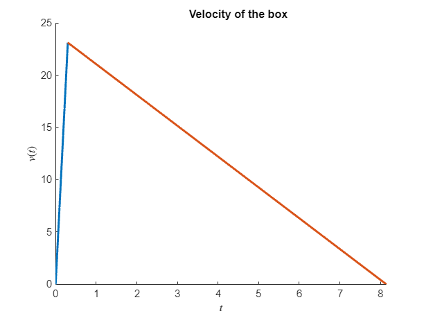
We can model this push as a linear force instead. Let us create a linear function for the load.
syms t1 t2 t
A = [1 t1
1 t2];
C = A\eye(2);
phi = simplify([1 t]*C);
P1Interp = phi*[sym('u1');sym('u2')]P1Interp = matlabFunction(P1Interp)P1Interp =
@(t,t1,t2,u1,u2)(u1.*(t-t2))./(t1-t2)-(u2.*(t-t1))./(t1-t2)P_lin = piecewise(t<0.15, P1Interp(t,0,0.15,0,4000), ...
t<0.3 , P1Interp(t,0.15,0.3,4000,0), ...
t>0.3 , 0)figure
fplot(P_lin,[0,2],'b')
xlabel('$t$ [s]','interpreter','latex')
ylabel('$P(t)$ [N]','interpreter','latex')
title('Piecewise linear load')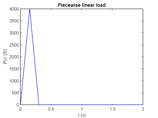
syms P
a_x = subs(a_x);
t1 = 0.15; t2 = 0.3;
DE1 = diff(x,t,2) == a_x;
x_dot = diff(x,t);
BV1 = [x(0) == 0, x_dot(0) == 0];
x1(t) = dsolve(DE1,BV1);
x1(t) = subs(x1, P, P1Interp(t,0,t1,0,4000))v1(t) = diff(x1,t)DE2 = diff(x,t,2) == a_x;
BV2 = [x(t1) == x1(t1), x_dot(t1) == v1(t1)];
x2(t) = dsolve(DE2,BV2);
x2(t) = subs(x2, P, P1Interp(t,t1,t2,4000,0))v2(t) = diff(x2,t)DE3 = diff(x,t,2) == subs(a_x,P,0);
BV3 = [x(t2) == x2(t2), x_dot(t2) == v2(t2)];
x3(t) = dsolve(DE3,BV3)v3(t) = diff(x3,t)t3 = double(solve(v3==0, t))t3 = 4.0733x_max = double(x3(t3))x_max = 24.4399figure;hold on
fplot(x1,[0,t1],'Linewidth',2)
fplot(x2,[t1,t2],'Linewidth',2)
fplot(x3,[t2,t3],'Linewidth',2)
xlabel('$t$','interpreter','latex')
ylabel('$x(t)$','interpreter','latex')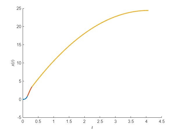
figure; hold on
fplot(v1,[0,t1],'Linewidth',2)
fplot(v2,[t1,t2],'Linewidth',2)
fplot(v3,[t2,t3],'Linewidth',2)
xlabel('$t$','interpreter','latex')
ylabel('$v(t)$','interpreter','latex')
title('Velocity of the box')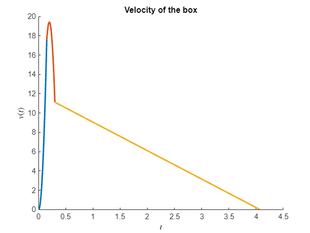
Comparing the two models, we note the significant difference in both velocity and sliding distance and for the case where the load is piece-wise linear, the box is starting to de-accelerate 0.15 seconds earlier.
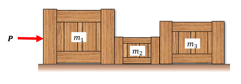
The three boxes are accelerated on the smooth surfaces by the force . Determine the motion and contact forces between the boxes.
Do determine the contact forces between the boxes we need to split the system up in three subsystems where we can apply Newton II och each individual box. Using Newton III on each subsystem we get the following situation with forces.
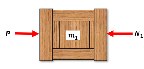
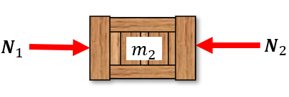
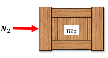
From these three subsystems, we formulate three kinetic equations as differential equations with the initial conditions stating that all three boxes have zero initial velocity and position.
clear
syms x1(t) x2(t) x3(t)
syms N1 N2 P m1 m2 m3
v1 = diff(x1,t); v2 = diff(x2,t); v3 = diff(x3,t);
a1 = diff(x1,t,2); a2 = diff(x2,t,2); a3 = diff(x3,t,2);

DE = [P - N1  == m1*a1
      N1 - N2 == m2*a2
      N2      == m3*a3];
BV = [v1(0)==0; x1(0)==0;
v2(0)==0; x2(0)==0;
v3(0)==0; x3(0)==0;];
s = dsolve(DE,BV);
x1 = s.x1x2 = s.x2x3 = s.x3To get the forces we need to couple the positions, creating two equations, from which we can solve for the forces.
[N1,N2] = solve([x1==x2, x2==x3], [N1,N2])A log with a mass kg is to be pulled up a ramp with a friction coefficient of using a pulley system according to the figure and a counter-mass of kg. The counter-mass travels 6 m, determine the velocity as it reaches the ground, starting from a resting position.

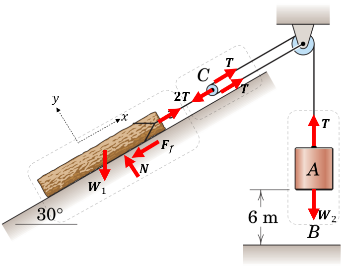
For the log we have:
For the counterweight we have:
clear
theta = 30;
syms m1 m2 g N mu_k T a_C a_A
F_W1 = m1*g*[-sind(theta); -cosd(theta)];
F_f = [-mu_k*N; 0];
F_N = [0; N];
F_T = [2*T; 0];
eq = F_W1 + F_f + F_T + F_N == m1*[a_C; 0]
eq = [eq;
      m2*g - T == m2*a_A]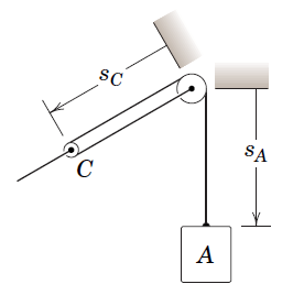
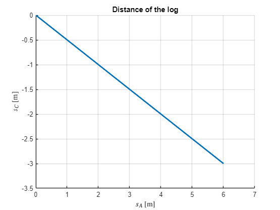
We begin by modeling the relation between the point and .
Note that the rope length is constant, let
syms s_C(t) s_A(t) L
eq = L == 2*s_C + s_AWe need to get and to use in the kinetics formulations. Let's differentiate L twice
diff(eq,t,2)We note that as increases, needs to decrease according to the geometric relation in the figure, thus we get:
The complete system of equations we need to deal with:
eq = [eq;
a_A == -2*a_C]Solving for the unknown variables
[T,N,a_C,a_A] = solve(eq, [T,N,a_C,a_A] )m1 = 200; m2 = 125; mu_k = 0.5; g=9.81;
T = double(subs(T))T = 707.9758N = double(subs(N))N = 1.6991e+03a_C = double(subs(a_C))a_C = -2.0731a_A = double(subs(a_A))a_A = 4.1462Now we can formulate the ODE
syms s_C(t)
v_A= diff(s_A,t);
s_A(t) = vpa(dsolve(diff(s_A,t,2) == a_A, v_A(0)==0, s_A(0)==0), 2)v_A(t) = diff(s_A,t)t1 = double(max(solve(s_A==6)))t1 = 1.7012v_A_end = vpa(v_A(t1),3)figure; hold on
fplot(s_A,[0,t1],'Linewidth',2)
plot(t1, s_A(t1),'o','MarkerFaceColor','k')
xlabel('$t$ [s]','interpreter','latex')
ylabel('$s_C(t)$ [m]','interpreter','latex')
title('Distance of the log')
grid on;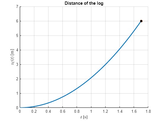
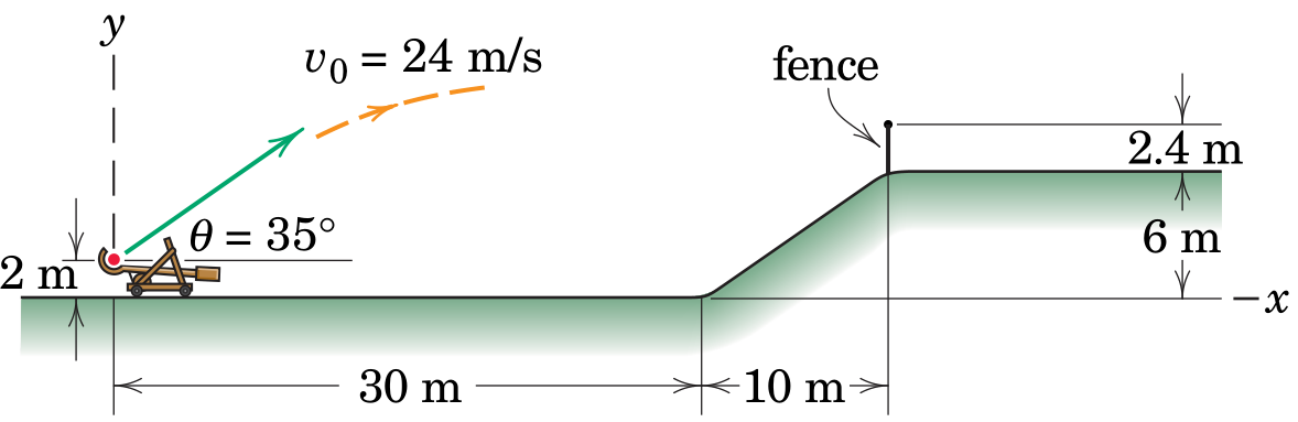
Plot the path of the projectile until it reaches the ground.
How long does the projectile hurl through the air?
How far away does the projectile impact ground?
What is the optimal angle to maximize the distance?
Add wind resistance according to , where is some geometric constant, is the velocity of the particle and is the velocity of the wind.
clear
v0 = 24;
theta = 35;
syms theta v0
V0 = v0*[cosd(theta); sind(theta)]syms x(t) y(t)
r(t) = [x(t); y(t)];
r_dot(t) = diff(r,t);
r_ddot = diff(r,t,2);
syms m g
DE = r_ddot*m == [0; -m*g]BV = [r_dot(0) == V0;
r(0) == [0;2]][x(t),y(t)] = dsolve(DE,BV)theta = 35; g = 9.82; v0 = 24; m = 4;
xn = subs(x); yn = subs(y);
t1 = double(max(solve(yn == 6)))t1 = 2.4744x1 = double(subs(xn,t,t1))x1 = 48.6457figure; hold on
fplot(xn,yn,[0,t1],'Displayname', '$\theta=35^\circ$');
hp = plot(NaN, NaN,'--r','Linewidth',2,'Displayname', ['$\theta=',num2str(0),'^\circ$']);
plot([0,30,40,250],[0,0,6,6],'-k','Handlevisibility','off')
plot([40,40],[6,8.4],'-k','Handlevisibility','off')
axis equal
axis([0,70,0,25])
xlabel('$x$ [m]','Interpreter','latex');
ylabel('$y$ [m]','Interpreter','latex');
% syms g v0 m theta
% xn = subs(x,[g,v0,m],[9.82, 24, 4])% yn = subs(y,[g,v0,m],[9.82, 24, 4])% xn = matlabFunction(xn);
% yn = matlabFunction(yn);
% tn = linspace(0,10,100);
% legend('show','Interpreter','latex')
% for thetan = [0:1:90, 89:-1:0]
% X = xn(tn, thetan);
% Y = yn(tn, thetan);
% set(hp,'XData',X,'YData',Y,'Displayname', ['$\theta=',num2str(thetan),'^\circ$'])
% drawnow
% end
Implementing a visualization we can quickly get a very good overview over the situation and graphically read the maximum height, distance, valid path etc.
To get the optimal angle to reach the maximum distance analytically we can get an expression for the time when the height is 6. Note that for some angles the particle never reaches this height, mathematically this is equivalent to not finding any roots, we need to be aware. We then substitute the expression for time into the expression for and plot the graph.
t2 = solve(yn==6, t)t2 = t2(2)xn = subs(x,[g,v0,m],[9.82, 24, 4])xn = formula(subs(xn, t, t2))figure
fplot(xn,[0,90])
xlabel('$\theta$ [deg]','Interpreter','latex');
ylabel('$x$ [m]','Interpreter','latex');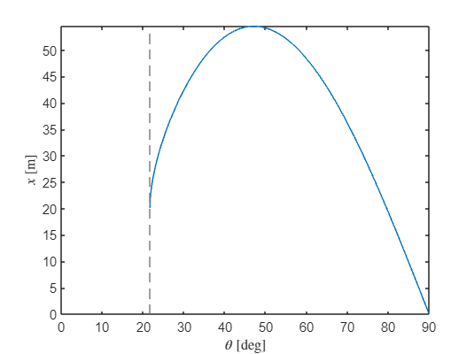
theta_max = double(vpasolve(diff(xn)==0,45))theta_max = 47.0985x_max = double(subs(xn,theta, theta_max))x_max = 54.5092The maximum distance is at 54 m and is reached by setting the launch angle to .
Adding wind resistance according to , where is some constant, is the velocity of the particle and is the velocity of the wind. We formulate the ODE
This becomes a non-linear ODE since we have to deal with the squared terms and which are the particles velocity. The sign is negative since the wind acts against the particle velocity. In addition to this, the surrounding air might actually have a velocity on its own, modeled by the vector . Here denotes a constant which actually is a combination of the drag coefficient, air density and the projectile cross-sectional area.
Let's set the wind velocity to
clear

syms theta v0
c = 0.03;
V0 = v0*[cosd(theta); sind(theta)]syms x(t) y(t)
r(t) = [x(t); y(t)];
r_dot(t) = diff(r,t);
r_ddot = diff(r,t,2);
v_W = [-2;0];
syms m g
DE = r_ddot*m == [0; -m*g] + c* -r_dot.^2 + v_WBV = [r_dot(0) == V0;
r(0) == [0;2]][x(t),y(t)] = dsolve(DE,BV)Warning: Unable to find symbolic solution.
x(t) =
[ empty sym ]
y(t) =
[ empty sym ]As we can see, dsolve is not able to find a symbolic solution, we need to tackle this numerically.
Applying Euler forward approximation we get
and similarly
From
we have
and
clear
v0 = 24; c = 0.03; theta = 47; m = 4; g = 9.82;
V0 = v0*[cosd(theta); sind(theta)];
v_W = [-20;22];

figure; hold on
hpath = plot(NaN, NaN,'-r','Linewidth',2,'Displayname', ['$\theta=',num2str(0),'^\circ$']);
hp = plot(NaN, NaN, 'ok','MarkerFaceColor','k');
plot([0,30,40,250],[0,0,6,6],'-k','Handlevisibility','off')
plot([40,40],[6,8.4],'-k','Handlevisibility','off')
axis equal; axis([0,70,0,25])
xlabel('$x$ [m]','Interpreter','latex');
ylabel('$y$ [m]','Interpreter','latex');
title(['$\theta=',num2str(theta),'^\circ, v_0=',num2str(v0), ...
    ' \mathrm{ m/s}, v_W=[',num2str(v_W(1)),',',num2str(v_W(2)),'] \mathrm{ m/s}$'], ...
    'interpreter','latex')

t = 0; dt = 0.1; i = 1;
vx = V0(1); vy = V0(2);
x = 0; y = 2;
X = NaN(100,1); Y = X;
while 1
    ax = (-c*vx^2 + c*sign(v_W(1))*v_W(1)^2)/m;
    ay = (-m*g -c*vy^2 + c*sign(v_W(2))*v_W(2)^2)/m;

    vx = vx + ax*dt;
    vy = vy + ay*dt;

    x = x + vx*dt;
    y = y + vy*dt;

    X(i) = x; Y(i) = y;
    set(hp,'XData',x,'YData',y)
    set(hpath,'XData',X,'YData',Y)
    % pause(0.1)
    drawnow

    t = t + dt; i = i + 1;
    if (x > 10 && y <= 0)
        break
    end
end
We note that even with no wind at all we can no longer make it over the obstacle, no matter what launch angle we choose, with the original initial velocity. We either need to make design changes to increase the initial velocity or hope for favorable winds.
Note that the parameter significantly affects the path, play around with the parameters!
Note how in general the path does not form a parabolic path which is why the swedish word "kastparabel" is very wrong to use.
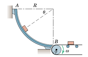
Small packages are released from rest at and slide down the smooth circular surface of radius to a conveyor at . Determine the expression for the the normal contact force between the guide and each package in terms of and specify the angular velocity of the conveyor wheel of radius to prevent any sliding on the belt as the object transitions from the circular path to the conveyor.
Solution: We start with the kinematics and describe the position of the package. With the origin according to the figure, we express the angle as a function of time and express the positin in Cartesion coordinates.
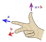
We state the normal and tangential directions next, and the tangential we can easily get by according to the right hand rule.
Then we can formulate the objects velocity and acceleration by differentiating the position vector.
clear
syms theta(t)
syms R r

e_R = [-cos(theta); -sin(theta); 0];
e_n = -e_R;
e_t = cross(e_n,[0;0;1])We get the position by
p = R*e_RThen the velocity
p_dot = subs(diff(p,t), diff(theta), sym('theta_dot'))And the acceleration
diff(p,t,2)p_ddot = subs(diff(p,t,2), [diff(theta,2), diff(theta)], ...
[sym('theta_ddot'), sym('theta_dot')])Now we can just project these onto the natural coordinates
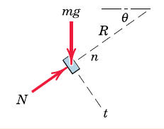
v_n = p_dot.' * e_nv_t = simplify(p_dot.' * e_t)a_n = simplify(p_ddot.' * e_n)a_t = simplify(p_ddot.' * e_t)Kinetics - From the free body diagram we get the forces
syms m g N
F_W = m*g*[0;-1;0]F_N = N*e_nWe want to convert these into natural coordinates as to state the equations of motion in natural coordinates
F_W_n = [F_W.' * e_n
F_W.' * e_t]F_N_n = [simplify(F_N.' * e_n)
F_N.' * e_t]We can now formulate the equations of motion
eq = F_W_n + F_N_n == m*[a_n
                         a_t];
And solve for the normal force as well as the angular acceleration
eq = formula(subs(eq, theta, 'theta'))[N,theta_ddot] = solve(eq, [N, 'theta_ddot'])Now to eliminate , we need to find out the angular velocity at , using we get
turns into:
and with and we have
where
syms v theta theta_dot
eq = int(v,v,0,v) == int(R*theta_ddot*R, theta, 0, theta)eq = subs(eq, v, R*theta_dot)theta_dot = solve(eq, theta_dot);
theta_dot = theta_dot(1)N = subs(N, 'theta_dot', theta_dot)Now, the geometric constraint means that the box needs to have the same speed as the conveyor belt, thus must hold! From this we can solve for
syms omega
theta_dot_2 = subs(theta_dot,theta,pi/2)omega = solve(omega*r == theta_dot_2*R, omega )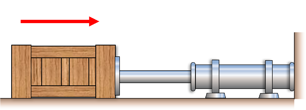
A box with a mass of is gliding without friction with a speed of when it hits a damper with a damping coefficient of . Determine the position and speed as a function of time.
Solution: We set the origin at the moment of impact. The only force acting of the box in the horizontal direction is the drag force for low velocity flow: . For high velocity the drag is proportional to the velocity squared. The distinction between low and high speed is given by the Reynolds number. Thus with Newton we have and the IVP becomes
We use dsolve to get the position as a function of time
clear
syms x(t) v0 m c

x_dot = diff(x,t);
DE = diff(x,2,t)*m == -c*x_dot;
BV = [x(0)==0; x_dot(0)==v0]x = dsolve(DE,BV)x_dot = diff(x,t)m = 1; c = 1; v0 = 1;
figure; hold on;
fplot(subs(x),[0,5],'LineWidth',2,'DisplayName','$x(t)$')
fplot(subs(x_dot),[0,5],'LineWidth',2,'DisplayName',"$x'(t)$")
legend('show','interpreter','latex')
xlabel('$t$','interpreter','latex');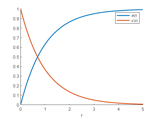
It is many times useful to express the velocity as a function of the position this can be done using the phase-plane. We can plot the parametric plot for a range, e.g.,
figure
fplot(subs(x_dot),subs(x),[0,5],'LineWidth',2,'DisplayName','$\dot{x}(x)$')
legend('show','interpreter','latex')
xlabel('$x(t)$','interpreter','latex');
ylabel('$\dot x(t)$','interpreter','latex')
title('Phase plane')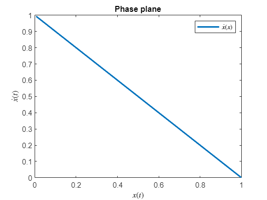
The alternative would be to first solve for in to get and plug this into which of course is more cumbersome, but we get an expression which can be analyzed.
t = solve(x==sym('x'), t)v_x = simplify(subs(x_dot))substitution gives
m = 1; c = 1; v0 = 1; syms x
subs(v_x)Then we plot
figure
fplot(subs(v_x),[0,1],'LineWidth',2,'DisplayName','$\dot{x}(x)$')
legend('show','interpreter','latex')
xlabel('$x(t)$','interpreter','latex');
ylabel('$\dot x(x)$','interpreter','latex')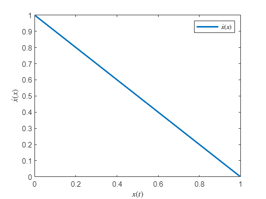
A spring and damper system is an extremely common model in dynamics.
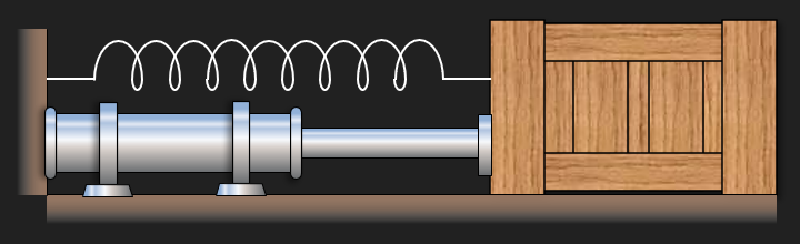
Schematically the system can be drawn like this
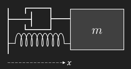
Free body diagram gives
where is an externally added force, is the spring coefficient and is the damping coefficient. The equation of motion is usually written on the form
For the following we shall assume zero external force for brevity. We have two options for initial values, either a nudge is given to the system in terms of an initial non-zero displacement
clear
syms x(t) c k m delta
v = diff(x,t);

DE = m*diff(x,2,t) + c*v + k*x == 0;
BV = [x(0)==delta; v(0)==0];
x = dsolve(DE,BV)Another option is to use an initial velocity
syms x(t) v0

BV = [x(0)==0; v(0)==v0];
x = dsolve(DE,BV)As we see we get a closed form solution for the position of the mass. This model is common enough to have special names and meaning attached to parts of the equation.
The standard form of the model is
where , is known as the natural frequency, is known as the damping ratio (zeta) and has special names associated with certain values, is undamped, is underdamped, is critically damped and is overdamped.
syms omega zeta u x(t) delta
v = diff(x,t);

DE = diff(x,2,t) + 2*zeta*omega*v + omega^2*x == 0;
BV = [x(0)==delta; v(0)==0];
x = simplify(dsolve(DE,BV))Setting some parameters to numerical values we can plot the oscillation
First undamped:
m = 1; k = 1; c = 0.0; delta = 0.1;
omega = sqrt(k/m)
omega = 1zeta = c/(2*m*omega)zeta = 0syms t
vpa(simplify(subs(x)),3)Here we can see that the solution is a cosine function with an constant amplitude of and the frequency of .
figure; hold on
fplot(subs(x),[0,10],'LineWidth',2,'Displayname',['$\zeta=',sprintf('%0.2f',zeta),'$'])
xlabel('$t$','interpreter','latex')
ylabel('$x(t)$','interpreter','latex')
legend('show','interpreter','latex')
Then we have underdamped
m = 1; k = 1; c = 0.5; delta = 0.1;
omega = sqrt(k/m)
omega = 1zeta = c/(2*m*omega)zeta = 0.2500vpa(simplify(subs(x)),3)fplot(subs(x),[0,10],'LineWidth',2,'Displayname',['$\zeta=',sprintf('%0.2f',zeta),'$'])Next we have a critically damped system
m = 1; k = 1;
omega = sqrt(k/m)
omega = 1c = 2.0000001; % Due to numerical instability
delta = 0.1;
zeta = c/(2*m*omega)zeta = 1.0000vpa(simplify(subs(x)),3)fplot(subs(x),[0,10],'LineWidth',2,'Displayname',['$\zeta=',sprintf('%0.2f',zeta),'$'])Finally an overdamped system
m = 1; k = 1;
omega = sqrt(k/m)
omega = 1c = 5;
delta = 0.1;
zeta = c/(2*m*omega)zeta = 2.5000vpa(simplify(subs(x)),3)fplot(subs(x),[0,10],'LineWidth',2,'Displayname',['$\zeta=',sprintf('%0.2f',zeta),'$'])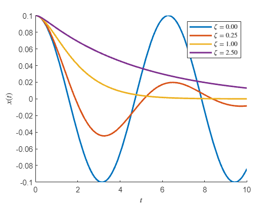
% This will plot the spring
% L = 5; b = 1; N = 20; delta = -1;
% y = linspace(L,0-delta,N+2);
% x = y*0+0;
% x(3:2:end-3) = x(3:2:end-3)-b/2;
% x(4:2:end-3) = x(4:2:end-3)+b/2;
%
% figure; hold on
% hSpring = plot(x,y,'k-');
% hMass = plot(x(end),y(end),'ko','MarkerFaceColor','k','MarkerSize',10);
% axis equal
% axis([-1,1,-L/2,L])
%
%
%
% syms omega zeta u x(t)
% v = diff(x,t);
% DE = diff(x,2,t) + 2*zeta*omega*v + omega^2*x == 0;
% BV = [x(0)==delta; v(0)==0];
% x = simplify(dsolve(DE,BV))%
% m = 1; k = 1; c = 5;
% omega = sqrt(k/m)omega = 1% zeta = c/(2*m*omega)zeta = 2.5000% syms t
% f = matlabFunction(simplify(subs(x)));
%
% title(['$\omega=1,\; \zeta=',sprintf('%0.2f',zeta),',\;\delta=1$'],'Interpreter','latex')
% xlabel('$t$','Interpreter','latex')
%
% t1 = 10; dt = 0.1;
% axis([-1,t1+1,-L/2,L])
% hPath = plot(NaN,NaN,'b-','LineWidth',2);
% X = NaN(length(t1/dt)); Y = X;
% i = 1;
% for t = 0:dt:t1
%
% y1 = f(t);
% y = linspace(L,0-y1,N+2);
% x = y*0+t;
% x(3:2:end-3) = x(3:2:end-3)-b/2;
% x(4:2:end-3) = x(4:2:end-3)+b/2;
% set(hSpring,'YData',y,'XData',x)
% set(hMass,'Ydata',y(end),'XData',x(end))
% X(i) = x(end); Y(i) = y(end);
% set(hPath,'Ydata',Y,'XData',X)
% drawnow
%
% append = true;
% if i == 1
% append = false;
% end
% exportgraphics(gca,"overdamped.gif","Append",append)
% i = i + 1;
%
% end

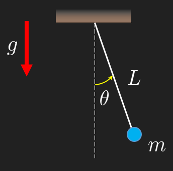
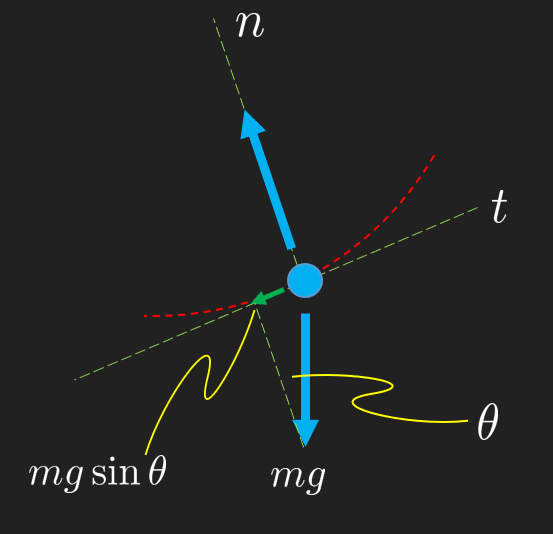
Thus
The arc length gives us
Thus we get the ODE for the simple pendulum
which is a non-linear ODE with no closed form solution. This needs to be solved using a numerical method for a given initial condition, e.g.,
For very small angles, , we can utilize the small angle approximation, and get a modified linear ODE
which for the above initial condition has the closed form solution